You are viewing the documentation for an older COMSOL version. The latest version is
available here.
The study step nodes’ Settings windows contain the following sections (in addition to specific study settings for each type of study step):
On top of the study steps Settings windows, a toolbar contains the following commands:
|
•
|
Click Compute (  ) or press F8 to compute the entire study. If there is an enabled Solver node under Solver Configurations, that solver sequence will be executed. Otherwise a new solver sequence will first be generated. See Computing a Solution.
|
Select the Include geometric nonlinearity check box to enable a geometrically nonlinear analysis for the study step. Some physics designs force a geometrically nonlinear analysis, in which case it is not possible to clear the
Include geometric nonlinearity check box. For further details, see the theory sections for the respective physics interface in the applicable modules’ manuals.
Select the Plot check box to allow plotting of results while solving in the
Graphics window. Then select what to plot from the
Plot group list and, for time-dependent simulations, at which time steps to update the plot: the output times or the time steps taken by the solver. The software plots the dataset of the selected plot group as soon as the results become available. You can also control which probes to tabulate and plot the values from. The default is to tabulate and plot the values from all probes in the
Table window and a
Probe Plot window.
Use the Probes list to select any probes to evaluate. The default is
All, which selects all probes for plotting and tabulation of probe data. Select
Manual to open a list with all available probes. Use the
Move Up (

),
Move Down (

),
Delete (

), and
Add (

) buttons to make the list contain the probes that you want to see results from while solving. Select
None to not include any probe.
See Physics and Variables Selection for detailed information about this section. You can control and specify different cases where the physics interface to solve for is varied, or, for various analysis cases, which variables and physics features (for example, boundary conditions and sources) to use. The default is to solve for all physics interfaces that are compatible with the study step type.
By default, the COMSOL Multiphysics software determines these values heuristically depending on the physics as, for example, the specified initial values or a solution from an earlier study step. Under Initial values of variables solved for, the default value of the
Settings list is
Physics controlled. To specify the initial values of the dependent variables that you solve for, select
User controlled from the
Settings list.
|
|
The Initial values of variables solved for settings have no effect when using the eigenvalue solver.
|
Then use the Method list to specify how to compute the initial values of variables solved for and the values of variables not solved for. Select:
|
•
|
Initial expression to use the expressions specified on the Initial Values nodes for the physics interface in the model.
|
|
•
|
Solution to use initial values as specified by a solution object (a solution from a study step).
|
Use the Study list to specify what study to use:
|
•
|
Select Zero solution to initialize all variables to zero.
|
Then use the Solution list to specify what solution object to use if
Study has been set to a study:
|
-
|
Current to use the current solution.
|
Depending on the solution object to use, you can choose different solutions to use. If a solution has nodes for storing solutions in its sequence, you can choose which solution to use using the Use list. The
Current value is the value that the solution has at the moment the value is read. The other values are the values stored in the respective nodes of the sequence. Choose
Manual to enter the index for the solution that you want to use. The index can be a global parameter that is swept in a Parametric sweep with solution number inputs to it.
For a Stationary study, from the
Selection list, select one of the following options:
|
•
|
Automatic (single solution) (the default) to select one solution on the Dependent Variables node depending on a global evaluation to find the current value of the parameters in the input solution or, if that is not possible, the last (typically the only) solution.
|
|
•
|
First to use the first (typically the only) solution
|
|
•
|
Last to use the last (typically the only) solution, select From list to pick solutions from a list.
|
|
•
|
Interpolated to specify an interpolated value in the text field below.
|
|
•
|
Manual to use a specific solution number that you specify in the Index field.
|
|
•
|
1 to use the first (typically the only) solution. If you use a parametric continuation of the stationary study, there can be additional solutions to choose from.
|
For a Time Dependent study, from the
Time list, select one of the following options:
|
•
|
Automatic (single solution) (the default) to select one solution on the Dependent Variables node depending on a global evaluation to find the current value of the parameters in the input solution or, if that is not possible, the solution for the last time.
|
|
•
|
First to use the first solution.
|
|
•
|
Last to use the last solution.
|
|
•
|
Manual to use a specific solution number that you specify in the Index field.
|
For an Eigenvalue or
Eigenfrequency study, from the
Eigenvalues list, select one of the following options:
|
•
|
Automatic (single solution) (the default) to select one solution on the Dependent Variables node depending on a global evaluation to find the current value of the parameters in the input solution or, if that is not possible, to use the solution for the first eigenvalue or eigenfrequency and its associated eigensolution.
|
|
•
|
First to use the first solution.
|
|
•
|
Last to use the last solution.
|
|
•
|
Interpolated to specify an eigenvalue of eigenfrequency in the text field below.
|
|
•
|
Manual to use a specific solution number that you specify in the Index field.
|
For a parametric or Frequency Domain study, from the
Parameter value list, select one of the following options:
|
•
|
Automatic (single solution) (the default) to select one solution on the Dependent Variables node depending on a global evaluation to find the current value of the parameters in the input solution or, if that is not possible, the solution for the last parameter value set or frequency.
|
|
•
|
First to use the first solution.
|
|
•
|
Last to use the last solution.
|
|
•
|
Manual to use a specific solution number that you specify in the Index field.
|
For the Automatic (all selections) option, all solutions are passed down to the solver, and the solver selects the initial values based on if there is a match to the current parameter tuple. This makes it possible to pass multiple initial values or guesses to the solver, which can be useful if you are doing a parametric study using multiple parameters and the convergence of each parameter tuple is dependent on a good initial guess. It can also be used together with the time-dependent parametric solver to use different initial values for each parameter tuple.
Under Store fields in output, you can specify to store the field variables that you solve only for some parts of the geometry (a boundary, for example, if the solution in the domain is not of interest). You define the parts of the geometry for which to store the fields as selection nodes. From the
Settings list, choose
All (the default) to store all fields in all parts of the geometry where they are defined, or choose
For selections to choose one or more selections that you add to the list. Click the
Add button (

) to open an
Add dialog box that contains all available selections. Select the selections that you want to add and then click
OK. You can also delete selections from the list using the
Delete button (

) and move them using the
Move Up (

) and
Move Down (

) buttons. See also the
Field node, where you can also control what to store in the output, if the corresponding
Dependent Variables uses user-defined settings.
|
|
If you use For selection and store the solution only for some parts of the geometry, it is not possible to continue with another study step.
|
Specify — for each geometry — which mesh to use for the study step. For each geometry listed in the Component column, select a mesh from the list of meshes in the
Mesh column. Each list of meshes contains the meshes defined for the geometry that you find on the same row.
These are settings for mesh adaptation and error estimates, available for stationary, eigenfrequency, eigenvalue, and frequency-domain study steps. Mesh adaptation (with other settings and operation) is also available for time-dependent study steps; see Time Dependent and
Adaptive Mesh Refinement (Time-Dependent Adaptation). Depending on the type of adaptation, meshing sequences for the adaptive mesh refinements, using
Adapt or
Size Expression nodes, and corresponding solutions are created for inspection and possible modification. Error estimates are available as variables for postprocessing (for example,
freq.errtot for the total error estimate in a Frequency Domain study). The adaptive mesh refinement solutions become available in a separate
Solution dataset (
Study 1/Adaptive Mesh Refinement Solutions 1, for example). When using that dataset for postprocessing, you can choose to use any of the available adaptive mesh refinement solutions from a
Parameter selection (Refinement level) list. Additional settings are available in the
Adaptive Mesh Refinement (Stationary and Eigenvalue Adaptation) and
Error Estimation subnodes under the solver node in the solver configurations.
From the Adaptation and error estimates list, select
Error estimates if you want to use error estimation or select
Adaptation and error estimates if you want to use adaptive mesh refinement. In the latter case, error estimates that are used in the adaptation algorithm are also available for postprocessing. Choose
None for no adaptation or error estimation. The internal name for the refinement level parameter is
adaptlevel. It is added by the adaptation solver method to separate the solutions for the different meshes. In the case that there is a user-defined parameter with that name in the model, a unique name for the refinement level parameter is made by adding a digit to
adaptlevel. You can use it to access the solutions from different mesh refinement levels using the
withsol() operator with; for example, using the following syntax:
withsol('sol1',expr,setval(adaptlevel,2)) to evaluate an expression
expr with the solution in
sol1 for the mesh adaptation level 2.
|
|
|
•
|
Adapt — the Adapt node in a meshing sequence also provides mesh adaptation. It includes a selection of geometric entities, which can be useful if you want to limit the mesh adaptation to certain geometric entities (some but not all domains, for example).
|
|
The software performs adaptive mesh refinement in one geometry only. Use the Adaptation in geometry list to specify that geometry. If you do not want to perform the mesh adaptation in the entire geometry, use the settings in the
Geometric Entity Selection for Adaptation section below.
Use the Error estimate list to control how the error estimate is computed:
|
•
|
Select L2 norm of error squared to use the squared L2 norm of the error. This is the only option for Eigenvalue studies. In the Error Estimation node under the Stationary Solver node, use the Scaling factor field to enter a space-separated list of scaling factors, one for each field variable (default: 1). The error estimate for each field variable is divided by this factor. Also, the L2 norm error estimate is based on a stability estimate for the PDE. Also in the Error Estimation node, use the Stability estimate derivative order field to specify its order (default: 2). For certain problems, which are symmetric and where strong error estimates hold, this method is equivalent to a functional error estimation with the functional being the L2 norm squared of the solution. This method can be used also for problems where these assumptions do not hold, but then the adaptation will not be optimal. See the following for some more in-depth information about these settings.
|
The L2 norm of error squared method estimates the error for a mesh element as a summation of contributions for the different equations solved for. It sums over

where A is the element area (volume, length),
h is the element size,
q is the
Stability estimate derivative order,
s is the
Scaling factor, and
ρ is an estimate of the PDE residual. The asymptotic behavior for
ρ is that it is proportional to
hp, where
p is the
Residual order (see below). Even if it is possible to estimate the actual value for
ρ very generally, assisting the algorithm with this order is important — for example, for the
Element selection method
Rough global minimum (in the
Adaptive Mesh Refinement subnode; see
Adaptive Mesh Refinement (Stationary and Eigenvalue Adaptation)), which essentially solves an optimization problem for where to refine so that the total error is reduced as much as possible (constrained by how many elements that can be added). All of the values for the
Stability estimate derivative order,
Scaling factor, and
Residual order (
q,
s, and
p, respectively, in the
Error Estimation subnode; see
Error Estimation) can all be given as vectors for the different equations. For the
Stability estimate derivative order, the default is 2, and it is related to the stability estimate that holds for the problem at hand. If it is not of a Poisson type, then it might need adjustment. For the
Scaling factor, the default is 1. It is mainly important to relatively weigh in the different parts of the equations solved for, which means that you need to give a space-separated array of numbers in general. Notice that when solving a multiphysics problem, the summation over different equations will not have the same unit since the different
ρ will have different units. So, a first effort with scaling would be to take this into account. In fact, not even a single-physics case like fluid flow will make this summation unit consistent because the residual for momentum and mass conservation will be added up with the default scaling factors of 1. For the
Residual order, the default is one order lower than the shape functions used for the equation. Change this only for nonstandard PDEs. Roughly speaking, the expected order is the basis order minus the highest spatial derivative order in the weak formulation. For a second-order PDE formulation with an integration by parts (lowering all second-order derivatives to first order) this will be of order one.
|
•
|
Select Functional and specify a Functional type. Available functional types are Predefined and Manual. This option adapts the mesh toward improved accuracy in the expression for the functional (for example, some energy, drag, or lift). Select Manual to specify a globally available scalar-valued expression in the Functional field (for example, the name of a global variable probe). If you select Predefined, you can choose from a predefined list of functional from the Solution functional list:
|
For a Stationary study step
stat, a global variable is defined for the functional with the name
stat.gfunc (and similarly for a frequency-domain study step). The functional can be evaluated under
Results>Derived Values by adding a
Global Evaluation node and, in the
Expressions section in its Settings window, selecting
Global Definitions>
Error estimation>stat.gfunc - Functional - Stationary.
The functional must be differentiable (or complex-valued analytic). Also, the expressions in the formulation must be differentiable. If this does not hold, the adjoint solution and its error estimate risk not being accurate, and the adaptation will then not be optimal for the functional used. The Functional option estimates the error for a mesh element as a summation of contributions. It sums over
A ωK ρ, where
ωK is computed from the adjoint (or dual) solution.
ωK can be computed with different methods (
PPR for Lagrange or
Interpolation error).
Equation 20-5 is about how
ωK is computed for
PPR for Lagrange. Notice that this method is not using scaling factors or the stability estimate derivative order because they are not part of the formula (they are built into
ωK). But
ρ is part of the formula and the residual order can therefore be important (for example, for the
Rough global minimum method; see
Adaptive Mesh Refinement (Stationary and Eigenvalue Adaptation)). For the
Approximate max norm, high order
p-norm. The reason for this is that it is possible to differentiate this functional.
|
•
|
Select Error indicator to specify an error indicator using an error expression, which you add to the Error expression table below using the Add (  ) button. The error expression can be any expression, including field variables and their derivatives, defined in the domain. This method will adapt the mesh where the error expression becomes large; the adaptation is typically not optimal. Select the Active check box for the error expressions that should be part of the error indicator. Use the Move Up (  ), Move Down (  ), and Delete (  ) buttons as needed to rearrange and remove error expressions. With this setting, there are no additional settings in the Error Estimation subnode, which becomes unavailable.
|
From the Add Error estimation variables list (not available if you chose
Error indicator from the
Error estimate list above), choose which variables to store, if any:
|
•
|
Select Error estimates and residuals to store all variables (the default).
|
|
•
|
Select Error estimates to store only the variables for error estimation.
|
|
•
|
Select None to not store any variables, which may lead to performance improvements.
|
The Save solution on every adapted mesh check box is selected per default. Clear this check box if you do not want to save solution on every adapted mesh. In that case, the last two solutions are saved (the finest one and the second finest) regardless of the total number of solutions.
Under Mesh adaptation, the following settings are available.
Use the Adaptation method list to control how to adaptively refine mesh elements. Select one of these methods:
|
•
|
General modification, to use the current mesh as a starting point and modify it by refinements, coarsening, topology modification, and point smoothing. Use the Allow coarsening check box to control if mesh coarsening is used. If the mesh contains anisotropic elements (for example, a boundary layer mesh), it is best to disable mesh coarsening to preserve the anisotropic structure. If you have selected to allow coarsening, specify the Maximum coarsening factor (a value of 5 by default) to scale the refined mesh size in the regions where refinement is not needed.
|
|
•
|
Rebuild mesh, to set up a size expression describing the error and rebuild the meshing sequence using the size expression as input. Note that structured meshes, such as mapped and swept meshes, in general are not appropriately refined. This method is not supported on imported meshes. The size of the refined mesh is the minimum of the size of the original mesh (previous refined mesh) and the size defined by the refinement. Specify the Maximum coarsening factor (a value of 3 by default) to scale the refined mesh size in the regions where refinement is not needed.
|
|
•
|
Regular refinement, to make the solver refine elements in a regular pattern by bisecting all edges of an element that needs refinement.
|
|
•
|
Longest edge refinement, to make the solver refine only the longest edge of an element by recursively bisecting the longest edge of edge elements that need refinement. This method is less suitable for models with nonsimplex elements. This is the default method.
|
With the settings in the Goal-oriented termination list you or the physics interfaces can add a number of global goal-oriented quantities so that the mesh adaptation will terminate when these are stable to a requested accuracy instead of after a fixed number of adaptation iterations. Choose
Off (the default),
Auto, or
Manual to control. You, when the list is set to
Manual, or the physics, when the list is set to
Auto, can add a number of global goal-oriented quantities, and the mesh adaptation will terminate when these are stable to a requested accuracy. These goal-oriented quantities could, for example, for an RF simulation be the S-parameters or another quantity of interest. The goal-oriented termination can be used with any of the available error estimation methods. When the
Goal-oriented termination list is set to
Manual, you can add goal-oriented terminal expressions in the table at the bottom of this section. Click the
Add button (

) to add an expression (default: 1) that you can edit in the
Goal-oriented termination expression column. If desired, adjust the tolerance (default: 0.01) in the
Tolerance column, and the type of tolerance in the
Tolerance type column:
Relative (the default) or
Absolute. Use the
Active buttons to manage which goal-oriented termination expressions to include. The mesh adaptation will run until the relative changes for all expressions (applied individually for all expressions) go below their respective thresholds, unless the maximum number of adaptations limit is met, in which case the algorithm terminates with a warning.
Use the Maximum number of adaptations field to specify the maximum number of adaptive mesh refinement iterations. The default value is 5 in 1D, 2 in 2D, and 1 in 3D. With the
Goal-oriented termination set to
Auto, the default value is set to 20 in 1D, 15 in 2D, and 10 in 3D.
With the Goal-oriented termination set to
Auto or
Manual, you can control the display of convergence from the adaptation when the
Output goal-oriented termination increments check box is selected. It is possible to choose the plot window to display the convergence as well as the table to be used by the plot from the
Plot window — select
New window (the default) or
Graphics — and
Output table lists, respectively. If you choose
New from the
Output table list, two new tables are created, one for the adaptation convergence plot and one for providing verbose information.
Also choose the level of detail for the log from the Goal-oriented termination log list:
Minimal,
Normal (the default), or
Detailed. Choose
Detailed if you want to include the evaluations for all the parameters, frequencies, or eigenvalues in the log.
From the Geometric entity level list, choose the geometric entity on which you want to do adaptive mesh refinement:
Entire geometry (the default),
Domain,
Boundary, or
Edge (3D only). For example, selecting
Boundary can be useful if the model includes a physics interface defined on boundaries (surfaces) and you want to base the adaptation on that physics interface. For all levels except
Entire geometry, select the geometric entities to include using the
Selection list and selection tools below.
Select the Auxiliary sweep check box to enable an auxiliary parameter sweep, which corresponds to a Parametric solver attribute node. For each set of parameter values, the chosen
Sweep type is solved for. This is available for Stationary, Time Dependent, and Frequency Domain studies.
Select a Sweep type to specify the type of sweep to perform:
|
•
|
Specified combinations (the default) solves for a number of given combinations of values as given for each parameter in the list. The parameter lists are combined in the order given, that is, the first combination contains the first value in each list, the second combination contains all second values, and so on.
|
|
•
|
All combinations solves for all combinations of values; that is, all values for each parameter are combined with all values for the other parameters. Using all combinations can lead to a very large number of solutions (equal to the product of the lengths of the parameter lists).
|
In the table, specify the Parameter name,
Parameter value list, and (optional)
Parameter unit for the parametric solver. Click the
Add button (

) to add a row to the table. When you click in the
Parameter value list column to define the parameter values, click the
Range button (

) to define a range of parameter values. The parameter unit overrides the unit of the global parameter. If no parameter unit is given, parameter values without explicit dimensions are considered dimensionless.
|
|
If you choose Specified combinations, the list of values must have equal length.
|
An alternative to specifying parameter names and values directly in the table is to specify them in a text file. Use the Load from File button (

) to browse to such a text file. The read names and values are appended to the current table. The format of the text file must be such that the parameter names appear in the first column and the values for each parameter appear row-wise with a space separating the name and values and a space separating the values.
Click the Save to File button (

) to save the contents of the table to a text file (or to a Microsoft Excel Workbook spreadsheet if the license includes LiveLink™
for Excel®).
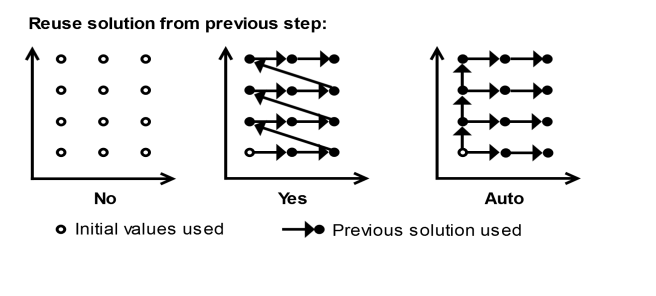
For a Stationary or Frequency Domain study, select an option from the Run continuation for list:
No parameter or one of the parameters given in the list.
|
•
|
No (the default for a Stationary study) to reset the solution to the initial values before each step or continuation sweep. The initial values will not be recalculated by the parametric solver for subsequent parameter values. Parameter dependence of the initial values can be accomplished by using parametric sweep.
|
|
•
|
Yes to always use the converged solution from the previous step, or the last solution from the previous continuation sweep (that is, never reset the solution).
|
|
•
|
Automatic (the default for a Frequency Domain study) to normally use the converged solution from the previous step or sweep. However, when multiple parameters are used, the solution from the first step of each parameter list is always used for the first step of the next list.
|
The difference between the three options is shown in Figure 20-2 for a 3-by-4 two-parameter sweep using the different choices for
Reuse solution from previous step without continuation:
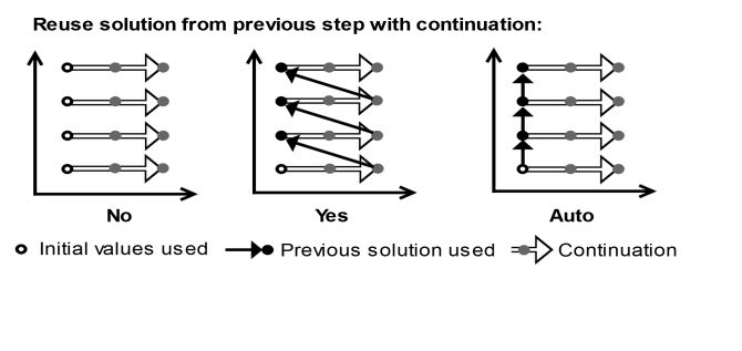
When continuation is enabled by setting Run continuation for to one of the parameters, the converged solutions are always reused for the steps along the continuation sweep in this parameter. The setting for
Reuse solution from previous step then determines how the solutions are reused between multiple continuation sweeps, if there are additional parameters to sweep over, as shown in
Figure 20-3.
For the Frequency Domain study, the auxiliary sweep is merged with the frequency sweep into a multiparameter sweep with the frequency as the parameter at the innermost level.