You are viewing the documentation for an older COMSOL version. The latest version is
available here.
An Adapt node (

) provides the possibility to use adaptive mesh refinement based on some error estimate from a computed solution. Adapt nodes are part of meshing sequences that the adaptive solver creates. You can also add
Adapt nodes by right-clicking a
Mesh node and select it from the
More Operations submenu. An
Adapt node modifies an existing mesh based on an expression, typically by refining the mesh based on error information from a solution.
The Adapt node’s
Settings window contains the following sections.
From the Geometric entity list, choose
Entire geometry (the default),
Domain,
Boundary, or
Edge to select a set of entities for which the adaptation is active. Choose
Manual in the
Selection list to select the entities in the Graphics window or choose a named selection to refer to a previously defined selection.
From the Solution list, select the solution to use for evaluation, or choose
None to not use any solution, but instead use the input mesh for the operation to evaluate on.
From the Solution selection list, select which solution that should be used to evaluate error estimates:
|
•
|
Select Use last to use the last solution.
|
|
•
|
Select Use first to use the first solution.
|
|
•
|
Select All (the default for Eigenvalue studies) to use all solutions from that study.
|
|
•
|
Select Manual to use a specific solution number that you specify as solution indices in the Index field.
|
In the Weights field (only available when
Solution selection is
Manual or
All), enter weights as a space-separated list of positive (relative) weights so that the error estimate is a weighted sum of the error estimates for the various solutions (eigenmodes). The default value is 1, which means that all the weight is put on the first solution (eigenmode). That is, any omitted weight components are treated as zero weight.
From the Type of expression list, choose
Error indicator (the default),
Absolute size, or
Anisotropic metric.
If you select Error indicator, the following settings appear:
The Error expression list, where you can add expressions for the error, for example, in terms of the dependent variables (including the variables for error estimation). You can use any expression, including field variables and their derivatives, defined in the domain. Use the
Active column to control which error expressions that are active by selecting or clearing the corresponding check box.
The Error order column is available when
Element selection is set to
Rough global minimum and forms an array of
h-exponents for the decrease of the error expression. This array has the same indexing as the error expression’s indexing (for an error expression with two expressions such as
errexpr1,
errexpr2 and error orders = 2, 3, it means that
errexpr1 =
O(
h2) and
errexpr2 =
O(
h3)). When the adaptation method is used, these numbers are filled in automatically based on the
Residual order and
Error estimate settings (on the adaptation study). The shape functions can also influence this order. Note that these order numbers need to be positive to generate additional elements (element growth).
Use the Move Up (

),
Move Down (

),
Add (

)and
Delete (

) buttons as needed. If you use several expressions, such as one for each solution component, the error expressions are added to form the sum of all of them. Or right-click a table cell and select
Move Up,
Move Down,
Add, or
Delete.
Use the Adaptation method list (2D and 3D only) to control how to adaptively refine mesh elements. Select one of these methods:
|
•
|
General modification, to use the current mesh as a starting point and modify it by refinements, coarsening, topology modification, and point smoothing. This is the default method. Use the Allow coarsening check box (selected by default) to control if mesh coarsening is used. If the mesh contains anisotropic elements (for example, a boundary layer mesh), it is best to disable mesh coarsening to preserve the anisotropic structure. If mesh coarsening is allowed, enter a Maximum coarsening factor (default: 5) if needed.
|
|
•
|
Regular refinement, to make the solver refine elements in a regular pattern by bisecting all edges of an element that needs refinement.
|
|
•
|
Longest edge refinement, to make the solver refine only the longest edge of an element by recursively bisecting the longest edge of edge elements that need refinement. This method is less suitable for models with nonsimplex elements.
|
Enter a value for the Maximum number of refinements (default: 5 in 2D and 3D; 16 in 1D), if needed.
Use the Element selection list to specify how the element refinement vector is determined from the error expression. Select:
|
•
|
Rough global minimum to minimize the L2 norm of the error by refining a fraction of the elements with the largest error in such a way that the total number of elements increases roughly by a factor greater than 1 specified in the accompanying Element count growth factor field. The default value is 1.7, which means that the number of elements increases by roughly 70%.
|
|
•
|
Fraction of worst error to refine elements whose local error indicator is larger than a given fraction of the largest local error indicator. Use the accompanying Element fraction field to specify the fraction. The default value is 0.5, which means that the fraction contains the elements with more than 50% of the largest local error.
|
|
•
|
Fraction of elements to refine a given fraction of the elements. Use the accompanying Element fraction field to specify the fraction. The default value is 0.5, which means that the solver refines about 50% of the elements with the largest local error indicator.
|
If you select Absolute size, the following settings appear:
In the Size expression field, type an expression for the element size (in terms of variables defined by the solution).
In 2D and 3D, use the Adaptation method list to control how to refine mesh elements. Select one of the following methods:
|
•
|
General modification, to use the current mesh as a starting point and modify it by refinements, coarsening, topology modification, and point smoothing. This is the default method. Use the Allow coarsening check box to control if mesh coarsening is used. If the mesh contains anisotropic elements (for example, a boundary layer mesh), it is best to disable mesh coarsening to preserve the anisotropic structure.
|
|
•
|
Regular refinement, to make the solver refine elements in a regular pattern by bisecting all edges of an element that needs refinement.
|
|
•
|
Longest edge refinement, to make the solver refine only the longest edge of an element by recursively bisecting the longest edge of edge elements that need refinement. This method is less suitable for models with nonsimplex elements.
|
If you select Anisotropic metric (2D and 3D only), the following settings appear:
In the matrix (2-by-2 in 2D; 3-by-3 in 3D) that appears, you can enter a metric in upper-triangular parts (the matrix is a positive definite symmetric matrix). The expressions for the metric can vary in space and include the local mesh element size h. The default value is a diagonal matrix with the diagonal elements set to
1/h, which means “no modification” for an isotropic mesh. The interpretation of the matrix is as follows: The vector representing an edge of an element is transformed by the matrix in that point, and the length of the transformed vector is measured. If the length is shorter than 1.0, it is considered too short. If it is longer than 1.0, it is considered too long. This measure is used to control the adaptation.
The following settings are available under External changes if the
Solution list is set to
None.
The selection in the Update when parameter is changed list provides the possibility to have the cache cleared whenever the values of the selected parameter are changed.
|
|
The Face representation setting is only available for 3D meshes that define their own geometric model. A typical example is a mesh imported from file.
|
|
•
|
Linear to place new or moved mesh vertices on the input mesh. A resulting refined mesh will keep the shape of the input mesh to a great extent, as seen in the upper right image in Figure 8-26.
|
|
•
|
Curved to place new or moved mesh vertices on a curved surface approximation of the input mesh. On curved faces where the mesh has been refined, the resulting mesh will typically be smoother than the input mesh, as seen in the lower right image in Figure 8-26. 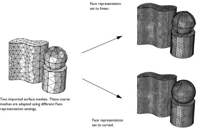
|