|
|
|
|
1
|
|
2
|
In the Select Physics tree, select Electrochemistry > Hydrogen Fuel Cells > Proton Exchange Membrane (fc).
|
|
3
|
Click Add.
|
|
4
|
Click
|
|
5
|
In the Select Study tree, select Preset Studies for Selected Physics Interfaces > Stationary with Initialization.
|
|
6
|
Click
|
|
1
|
|
2
|
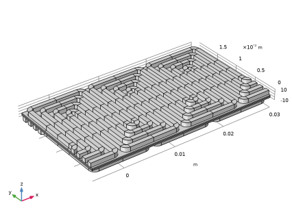
Browse to the model’s Application Libraries folder and double-click the file pemfc_serpentine_flow_field_geom_sequence.mph.
|
|
3
|
|
4
|
|
1
|
|
2
|
|
3
|
Locate the Parameters section. In the table, enter the following settings:
|
|
1
|
|
2
|
|
3
|
|
4
|
|
1
|
|
2
|
|
3
|
|
4
|
Browse to the model’s Application Libraries folder and double-click the file pemfc_serpentine_flow_field_physics_parameters.txt.
|
|
1
|
|
2
|
Go to the Add Material window.
|
|
3
|
In the tree, select Fuel Cell and Electrolyzer > Polymer Electrolytes > Nafion®, EW 1100, Vapor Equilibrated, Protonated.
|
|
4
|
Right-click and choose Add to Component 1 (comp1).
|
|
5
|
|
1
|
|
2
|
Find the Transport mechanisms subsection. Select the Use Darcy’s Law for momentum transport checkbox.
|
|
3
|
|
1
|
In the Model Builder window, expand the Component 1 (comp1) > Geometry 1 node, then click Component 1 (comp1) > Hydrogen Fuel Cell (fc) > Membrane 1.
|
|
2
|
|
3
|
|
1
|
|
2
|
|
3
|
Select the Electroosmotic water drag checkbox.
|
|
1
|
In the Model Builder window, under Component 1 (comp1) > Hydrogen Fuel Cell (fc) > Membrane 1 click Initial Values 1.
|
|
2
|
|
3
|
|
4
|
|
1
|
|
2
|
In the Settings window for Water Absorption-Desorption, H2 Side, locate the Absorption-Desorption Condition section.
|
|
3
|
|
1
|
|
2
|
In the Settings window for Water Absorption-Desorption, O2 Side, locate the Absorption-Desorption Condition section.
|
|
3
|
|
1
|
|
2
|
|
3
|
|
4
|
|
5
|
|
6
|
|
7
|
|
1
|
|
2
|
|
3
|
|
4
|
|
5
|
|
6
|
|
7
|
|
1
|
|
2
|
|
3
|
|
4
|
|
5
|
|
6
|
|
1
|
|
2
|
|
3
|
|
4
|
|
5
|
|
6
|
|
1
|
|
2
|
|
3
|
|
4
|
|
1
|
|
2
|
In the Settings window for Thin H2 Gas Diffusion Electrode Reaction, locate the Electrode Kinetics section.
|
|
3
|
|
4
|
|
1
|
|
2
|
|
3
|
|
4
|
|
1
|
|
2
|
In the Settings window for Thin O2 Gas Diffusion Electrode Reaction, locate the Electrode Kinetics section.
|
|
3
|
|
4
|
|
5
|
|
1
|
|
2
|
|
3
|
|
1
|
|
2
|
|
3
|
|
4
|
|
5
|
|
1
|
|
2
|
|
3
|
|
4
|
|
5
|
|
6
|
|
1
|
In the Model Builder window, under Component 1 (comp1) > Hydrogen Fuel Cell (fc) > H2 Gas Phase 1 click Initial Values 1.
|
|
2
|
|
3
|
|
1
|
|
2
|
|
3
|
|
4
|
|
5
|
|
6
|
|
7
|
|
8
|
|
1
|
|
2
|
|
3
|
|
1
|
In the Model Builder window, under Component 1 (comp1) > Hydrogen Fuel Cell (fc) > O2 Gas Phase 1 click Initial Values 1.
|
|
2
|
|
3
|
|
4
|
|
1
|
|
2
|
|
3
|
|
4
|
|
5
|
|
6
|
|
7
|
|
8
|
|
9
|
|
10
|
|
1
|
|
2
|
|
3
|
|
1
|
|
2
|
|
3
|
|
4
|
|
1
|
|
2
|
|
3
|
|
1
|
|
2
|
|
3
|
|
1
|
|
2
|
|
3
|
|
4
|
|
5
|
|
6
|
|
7
|
Select the Symmetric distribution checkbox.
|
|
1
|
|
2
|
|
3
|
|
4
|
|
1
|
|
2
|
|
3
|
Click the Custom button.
|
|
4
|
Locate the Element Size Parameters section.
|
|
5
|
|
6
|
|
1
|
|
2
|
|
3
|
|
4
|
|
1
|
|
2
|
|
3
|
|
4
|
|
1
|
|
2
|
|
3
|
|
4
|
|
1
|
|
2
|
|
3
|
|
4
|
|
5
|
|
6
|
|
7
|
|
1
|
|
2
|
|
3
|
|
4
|
|
1
|
|
2
|
|
3
|
Click the Custom button.
|
|
4
|
Locate the Element Size Parameters section.
|
|
5
|
|
6
|
|
1
|
|
2
|
|
3
|
|
4
|
|
1
|
|
2
|
|
3
|
|
4
|
|
5
|
|
6
|
|
1
|
|
2
|
|
3
|
|
1
|
|
2
|
|
1
|
|
2
|
|
3
|
|
4
|
Click
|
|
1
|
|
2
|
|
3
|
|
4
|
|
5
|
In the Model Builder window, expand the Study 1 > Solver Configurations > Solution 1 (sol1) > Dependent Variables 2 node, then click Chemical Potential (comp1.fc.mu0).
|
|
6
|
|
7
|
Clear the Solve for this field checkbox.
|
|
8
|
In the Model Builder window, under Study 1 > Solver Configurations > Solution 1 (sol1) > Dependent Variables 2 click Electrolyte Potential (comp1.fc.phil).
|
|
9
|
|
10
|
Clear the Solve for this field checkbox.
|
|
11
|
In the Model Builder window, under Study 1 > Solver Configurations > Solution 1 (sol1) > Dependent Variables 2 click Electric Potential (comp1.fc.phis).
|
|
12
|
|
13
|
Clear the Solve for this field checkbox.
|
|
14
|
In the Model Builder window, under Study 1 > Solver Configurations > Solution 1 (sol1) > Dependent Variables 2 click Mass Fraction (comp1.fc.wH2O_H2).
|
|
15
|
|
16
|
Clear the Solve for this field checkbox.
|
|
17
|
In the Model Builder window, under Study 1 > Solver Configurations > Solution 1 (sol1) > Dependent Variables 2 click Mass Fraction (comp1.fc.wH2O_O2).
|
|
18
|
|
19
|
Clear the Solve for this field checkbox.
|
|
20
|
In the Model Builder window, under Study 1 > Solver Configurations > Solution 1 (sol1) > Dependent Variables 2 click Mass Fraction (comp1.fc.wN2_O2).
|
|
21
|
|
22
|
Clear the Solve for this field checkbox.
|
|
23
|
In the Model Builder window, under Study 1 > Solver Configurations > Solution 1 (sol1) > Dependent Variables 2 click Electric Potential on Boundary (comp1.fc.ecph1.ec1.phis0).
|
|
24
|
|
25
|
Clear the Solve for this state checkbox.
|
|
26
|
In the Model Builder window, under Study 1 > Solver Configurations > Solution 1 (sol1) > Dependent Variables 2 click Boundary Mass Fraction (comp1.fc.h2gasph1.h2in1.wbndH2O).
|
|
27
|
|
28
|
Clear the Solve for this state checkbox.
|
|
29
|
In the Model Builder window, under Study 1 > Solver Configurations > Solution 1 (sol1) > Dependent Variables 2 click Boundary Mass Fraction (comp1.fc.o2gasph1.o2in1.wbndH2O).
|
|
30
|
|
31
|
Clear the Solve for this state checkbox.
|
|
32
|
In the Model Builder window, under Study 1 > Solver Configurations > Solution 1 (sol1) > Dependent Variables 2 click Boundary Mass Fraction (comp1.fc.o2gasph1.o2in1.wbndN2).
|
|
33
|
|
34
|
Clear the Solve for this state checkbox.
|
|
35
|
|
36
|
|
1
|
|
2
|
|
3
|
Clear the Plot dataset edges checkbox.
|
|
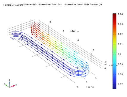
1
|
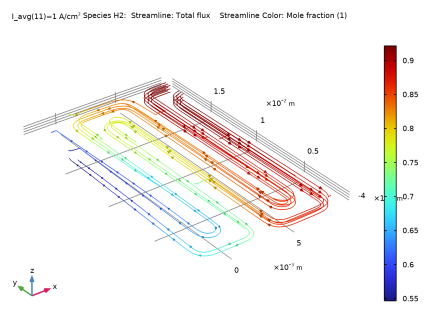
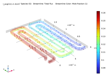
In the Model Builder window, expand the Mole Fraction, H2, Streamline (fc) node, then click Streamline 1.
|
|
2
|
|
3
|
|
4
|
|
5
|
Locate the Coloring and Style section. Find the Point style subsection. From the Arrow distribution list, choose Equal time.
|
|
6
|
|
1
|
|
2
|
|
3
|
Clear the Plot dataset edges checkbox.
|
|
1
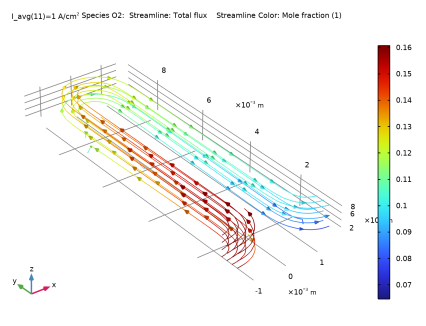
|
In the Model Builder window, expand the Mole Fraction, O2, Streamline (fc) node, then click Streamline 1.
|
|
2
|
|
3
|
|
4
|
|
5
|
Locate the Coloring and Style section. Find the Point style subsection. From the Arrow distribution list, choose Equal time.
|
|
6
|
|
1
|
|
2
|
|
1
|
|
2
|
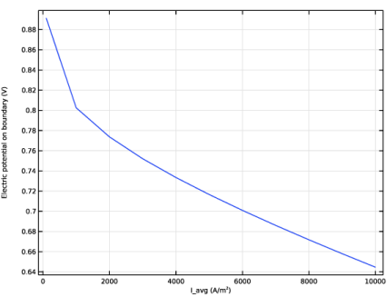
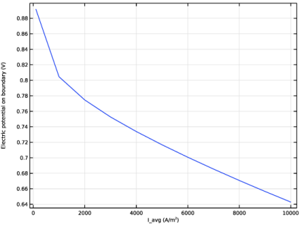
In the Settings window for Global, click Replace Expression in the upper-right corner of the y-Axis Data section. From the menu, choose Component 1 (comp1) > Hydrogen Fuel Cell > fc.phis0_ec1 - Electric potential on boundary - V.
|
|
1
|
|
2
|
|
3
|
|
4
|
|
5
|
|
1
|
|
2
|
|
3
|
|
4
|
|
5
|
|
1
|
|
2
|
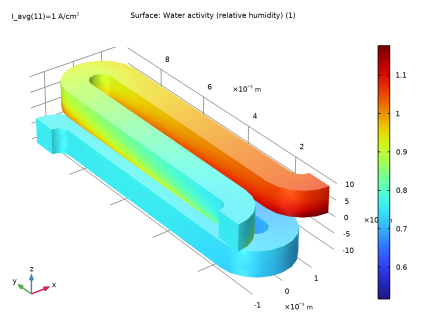
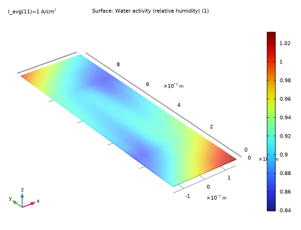
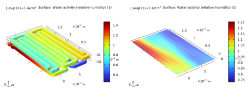
In the Settings window for Surface, click Replace Expression in the upper-right corner of the Expression section. From the menu, choose Component 1 (comp1) > Hydrogen Fuel Cell > fc.aw - Water activity (relative humidity) - 1.
|
|
3
|
|
1
|
|
2
|
|
3
|
|
4
|
|
1
|
|
2
|
In the Settings window for Surface, click Replace Expression in the upper-right corner of the Expression section. From the menu, choose Component 1 (comp1) > Hydrogen Fuel Cell > Membrane transport > fc.aw_mem - Water activity (relative humidity) - 1.
|
|
3
|
|
1
|
|
2
|
|
1
|
|
2
|
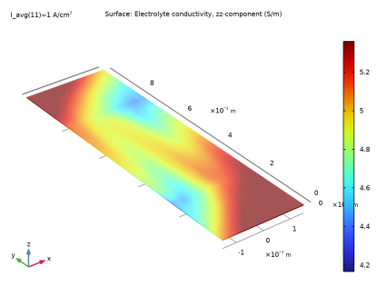
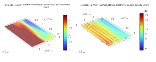
In the Settings window for Surface, click Replace Expression in the upper-right corner of the Expression section. From the menu, choose Component 1 (comp1) > Hydrogen Fuel Cell > Electrolyte conductivity - S/m > fc.sigmalzz - Electrolyte conductivity, zz-component.
|
|
3
|
|
1
|
|
2
|
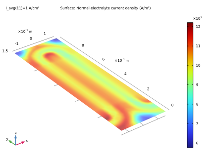
In the Settings window for 3D Plot Group, type Cross-Membrane Current Density in the Label text field.
|
|
3
|
|
1
|
|
2
|
In the Settings window for Surface, click Replace Expression in the upper-right corner of the Expression section. From the menu, choose Component 1 (comp1) > Hydrogen Fuel Cell > fc.nIl - Normal electrolyte current density - A/m².
|
|
3
|
|
1
|
|
2
|
|
3
|
|
1
|
|
2
|
|
3
|
|
4
|
|
1
|
|
2
|
|
1
|
|
2
|
|
3
|
|
1
|
|
2
|
|
1
|
In the Model Builder window, under Study 1 > Solver Configurations right-click Solution 1 (sol1) and choose Solution > Copy.
|
|
1
|
In the Model Builder window, under Study 1 > Solver Configurations click Solution 1 - Copy 1 (sol4).
|
|
2
|
|
1
|
|
2
|
|
3
|
|
4
|
|
5
|
|
6
|
In the Model Builder window, expand the Study 1 > Solver Configurations > Solution 1 (sol1) > Dependent Variables 2 node, then click Chemical Potential (comp1.fc.mu0).
|
|
7
|
|
8
|
Clear the Solve for this field checkbox.
|
|
9
|
|
10
|
|
11
|
Clear the Solve for this field checkbox.
|
|
12
|
|
13
|
|
14
|
Clear the Solve for this field checkbox.
|
|
15
|
|
16
|
|
17
|
Clear the Solve for this field checkbox.
|
|
18
|
|
19
|
|
20
|
Clear the Solve for this field checkbox.
|
|
21
|
|
22
|
|
23
|
Clear the Solve for this field checkbox.
|
|
24
|
|
25
|
|
26
|
Clear the Solve for this state checkbox.
|
|
27
|
|
28
|
|
29
|
Clear the Solve for this state checkbox.
|
|
30
|
|
31
|
|
32
|
Clear the Solve for this state checkbox.
|
|
33
|
|
34
|
|
35
|
Clear the Solve for this state checkbox.
|
|
1
|
|
2
|
|
3
|
Select the Plot checkbox.
|
|
4
|
|
5
|