|
|
|

|
1
|
|
2
|
|
3
|
Click Add.
|
|
4
|
Click
|
|
5
|
In the Select Study tree, select Preset Studies for Selected Physics Interfaces > Stationary with Initialization.
|
|
6
|
Click
|
|
1
|
|
2
|
Browse to the model’s Application Libraries folder and double-click the file soec_geom_sequence.mph.
|
|
3
|
|
4
|
|
1
|
|
2
|
|
1
|
|
2
|
|
3
|
|
4
|
Browse to the model’s Application Libraries folder and double-click the file soec_physics_parameters.txt.
|
|
1
|
|
2
|
|
3
|
Click
|
|
5
|
Locate the H2 Gas Mixture section. Find the Transport mechanisms subsection. Clear the Include gas phase diffusion checkbox.
|
|
1
|
|
1
|
|
2
|
Go to the Add Material window.
|
|
3
|
In the tree, select Fuel Cell and Electrolyzer > Solid Oxides > Yttria-Stabilized Zirconia, 8YSZ, (ZrO2)0.92-(Y2O3)0.08.
|
|
4
|
Right-click and choose Add to Component 1 (comp1).
|
|
5
|
|
1
|
|
2
|
|
3
|
|
4
|
|
5
|
|
1
|
|
2
|
In the Settings window for H2 Gas Diffusion Electrode Reaction, locate the Electrode Kinetics section.
|
|
3
|
|
4
|
|
1
|
|
2
|
|
3
|
|
4
|
|
5
|
|
1
|
|
2
|
In the Settings window for O2 Gas Diffusion Electrode Reaction, locate the Electrode Kinetics section.
|
|
3
|
|
4
|
|
1
|
In the Model Builder window, under Component 1 (comp1) > Water Electrolyzer (we) click Electronic Conducting Phase 1.
|
|
1
|
|
2
|
|
3
|
|
4
|
|
5
|
|
1
|
|
2
|
|
3
|
From the list, choose Average current density.
|
|
4
|
|
5
|
|
6
|
|
7
|
|
1
|
|
2
|
|
3
|
|
4
|
|
1
|
|
2
|
|
3
|
|
4
|
Locate the Element Size Parameters section.
|
|
5
|
|
1
|
|
2
|
|
3
|
|
5
|
|
1
|
|
2
|
|
3
|
|
5
|
|
1
|
|
2
|
|
3
|
|
4
|
|
1
|
|
2
|
|
3
|
|
4
|
|
5
|
|
6
|
|
7
|
|
8
|
Click
|
|
1
|
|
2
|
|
3
|
|
4
|
|
1
|
|
2
|
|
3
|
Click
|
|
5
|
|
6
|
|
7
|
Select the Reverse direction checkbox.
|
|
1
|
|
2
|
|
3
|
Click
|
|
5
|
|
1
|
In the Model Builder window, under Component 1 (comp1) > Mesh 1 > Swept 2 right-click Distribution 1 and choose Duplicate.
|
|
2
|
|
3
|
Click
|
|
5
|
|
6
|
|
1
|
|
1
|
|
1
|
|
2
|
Go to the Add Physics window.
|
|
3
|
In the tree, select Fluid Flow > Porous Media and Subsurface Flow > Free and Porous Media Flow, Brinkman (fp).
|
|
4
|
Click the Add to Component 1 button in the window toolbar.
|
|
5
|
|
2
|
In the Settings window for Free and Porous Media Flow, Brinkman, locate the Domain Selection section.
|
|
3
|
Click
|
|
4
|
|
5
|
Click OK.
|
|
6
|
|
7
|
|
1
|
|
2
|
|
3
|
|
1
|
|
2
|
|
3
|
|
4
|
|
1
|
|
2
|
|
3
|
|
4
|
|
5
|
|
1
|
|
2
|
|
3
|
|
4
|
|
1
|
|
2
|
|
3
|
|
4
|
Locate the H2 Gas Mixture section. Find the Transport mechanisms subsection. Select the Include gas phase diffusion checkbox.
|
|
1
|
|
2
|
|
3
|
|
1
|
|
2
|
|
3
|
|
4
|
Select the Include pore-wall interaction checkbox.
|
|
5
|
|
1
|
|
1
|
|
2
|
|
3
|
|
4
|
|
5
|
|
1
|
|
2
|
|
3
|
|
1
|
|
2
|
|
3
|
|
1
|
|
2
|
In the Settings window for Current Distribution Initialization, locate the Physics and Variables Selection section.
|
|
3
|
In the Solve for column of the table, under Component 1 (comp1) > Multiphysics, clear the checkbox for Reacting Flow, H2 Gas Phase 1 (rfh1).
|
|
1
|
|
2
|
|
3
|
In the Solve for column of the table, under Component 1 (comp1), clear the checkbox for Water Electrolyzer (we).
|
|
4
|
In the Solve for column of the table, under Component 1 (comp1) > Multiphysics, clear the checkbox for Reacting Flow, H2 Gas Phase 1 (rfh1).
|
|
1
|
|
1
|
|
2
|
|
3
|
In the Model Builder window, expand the Study 1 > Solver Configurations > Solution 1 (sol1) > Stationary Solver 3 node.
|
|
4
|
|
5
|
|
1
|
|
2
|
|
3
|
|
4
|
|
5
|
|
6
|
|
1
|
|
2
|
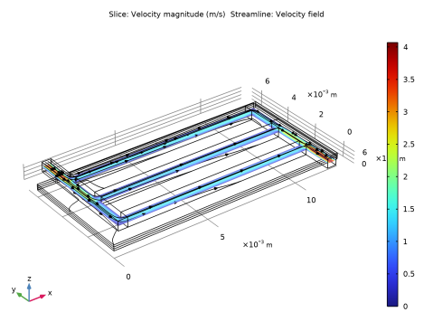
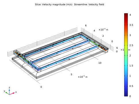
In the Settings window for Streamline, click Replace Expression in the upper-right corner of the Expression section. From the menu, choose Component 1 (comp1) > Free and Porous Media Flow, Brinkman > Velocity and pressure > u,v,w - Velocity field.
|
|
3
|
|
4
|
Locate the Coloring and Style section. Find the Point style subsection. From the Type list, choose Arrow.
|
|
5
|
|
6
|
|
7
|
|
1
|
|
2
|
|
1
|
|
2
|
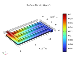
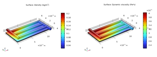
In the Settings window for Surface, click Replace Expression in the upper-right corner of the Expression section. From the menu, choose Component 1 (comp1) > Free and Porous Media Flow, Brinkman > Material properties > fp.rho - Density - kg/m³.
|
|
3
|
|
1
|
|
2
|
|
1
|
|
2
|
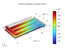
In the Settings window for Surface, click Replace Expression in the upper-right corner of the Expression section. From the menu, choose Component 1 (comp1) > Free and Porous Media Flow, Brinkman > Material properties > fp.mu - Dynamic viscosity - Pa·s.
|
|
3
|
|
1
|
|
1
|
|
2
|
|
3
|
|
1
|
|
2
|
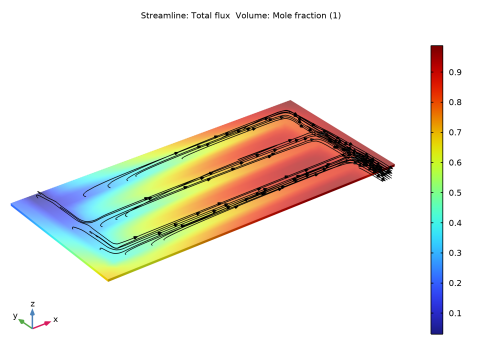
In the Settings window for Streamline, click Replace Expression in the upper-right corner of the Expression section. From the menu, choose Component 1 (comp1) > Water Electrolyzer > Species H2 > we.tfluxH2x,...,we.tfluxH2z - Total flux.
|
|
3
|
|
4
|
|
5
|
Locate the Coloring and Style section. Find the Point style subsection. From the Type list, choose Arrow.
|
|
6
|
|
7
|
|
1
|
|
2
|
|
3
|
|
1
|
|
2
|
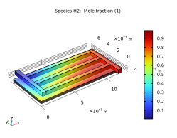
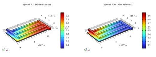
In the Settings window for Volume, click Replace Expression in the upper-right corner of the Expression section. From the menu, choose Component 1 (comp1) > Water Electrolyzer > Species H2 > we.xH2 - Mole fraction - 1.
|
|
1
|
|
2
|
|
3
|
|
4
|
|
5
|
|
1
|
|
2
|
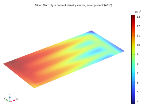
In the Settings window for 3D Plot Group, type Cross-Sectional Electrolyte Current Density in the Label text field.
|
|
3
|
|
1
|
|
2
|
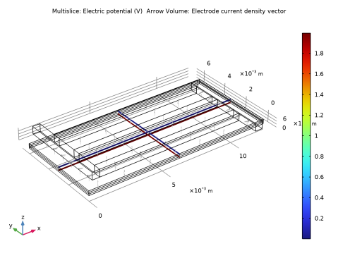
In the Settings window for Slice, click Replace Expression in the upper-right corner of the Expression section. From the menu, choose Component 1 (comp1) > Water Electrolyzer > Electrolyte current density vector - A/m² > we.Ilz - Electrolyte current density vector, z-component.
|
|
3
|
|
4
|
|
5
|
|
6
|
|
1
|
|
2
|
Click
|
|
1
|
|
2
|
|
3
|
|
4
|
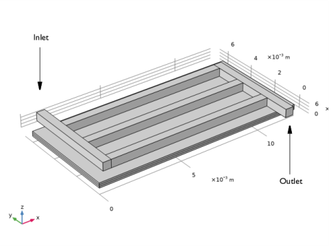
Browse to the model’s Application Libraries folder and double-click the file soec_geom_parameters.txt.
|
|
1
|
|
2
|
|
3
|
|
4
|
|
5
|
|
6
|
Locate the Selections of Resulting Entities section. Select the Resulting objects selection checkbox.
|
|
1
|
|
2
|
|
3
|
|
1
|
|
2
|
|
3
|
|
1
|
|
2
|
|
3
|
|
1
|
|
2
|
|
3
|
|
4
|
|
5
|
|
6
|
|
1
|
Right-click Component 1 (comp1) > Geometry 1 > Work Plane 1 (wp1) > Plane Geometry > Rectangle 1 (r1) and choose Duplicate.
|
|
2
|
|
3
|
|
4
|
|
1
|
|
2
|
|
3
|
|
4
|
|
5
|
|
6
|
|
1
|
|
2
|
Select the object r3 only.
|
|
3
|
|
4
|
|
5
|
|
6
|
|
1
|
|
2
|
|
3
|
Locate the Distances section. In the table, enter the following settings:
|
|
4
|
Locate the Selections of Resulting Entities section. Select the Resulting objects selection checkbox.
|
|
1
|
|
2
|
|
3
|
|
4
|
On the object fin, select Boundary 19 only.
|
|
1
|
|
2
|
|
3
|
|
4
|
On the object fin, select Boundary 42 only.
|
|
1
|
|
2
|
In the Settings window for Explicit Selection, type Cathode Current Collector in the Label text field.
|
|
3
|
|
4
|
On the object fin, select Boundaries 10, 26, 33, and 40 only.
|
|
1
|
|
2
|
In the Settings window for Explicit Selection, type Anode Current Collector in the Label text field.
|
|
3
|
|
4
|
On the object fin, select Boundary 3 only.
|
|
1
|
|
2
|
|
3
|
Click
|
|
4
|
|
5
|
Click OK.
|
|
6
|
In the Settings window for Adjacent Selection, type Channel Domain Boundaries in the Label text field.
|
|
1
|
|
2
|
In the Settings window for Difference Selection, type Boundary Layer Boundaries in the Label text field.
|
|
3
|
|
4
|
|
5
|
|
6
|
Click OK.
|
|
7
|
|
8
|
|
9
|
|
10
|
Click OK.
|