|
|
|


|
1
|
|
2
|
In the Application Libraries window, select Battery Design Module > Lithium-Ion Batteries, Performance > lib_base_model_1d in the tree.
|
|
3
|
Click
|
|
1
|
|
2
|
|
1
|
|
2
|
|
3
|
|
4
|
Browse to the model’s Application Libraries folder and double-click the file lib_internal_resistance_parameters.txt.
|
|
1
|
|
2
|
Go to the Add Physics window.
|
|
3
|
|
4
|
Click the Add to Component 1 button in the window toolbar.
|
|
5
|
|
1
|
|
2
|
|
1
|
|
2
|
|
3
|
|
4
|
|
5
|
|
6
|
Locate the Reinitialization section. In the table, enter the following settings:
|
|
1
|
|
2
|
|
3
|
|
4
|
|
5
|
|
6
|
Locate the Reinitialization section. In the table, enter the following settings:
|
|
1
|
In the Model Builder window, expand the Component 1 (comp1) > Definitions node, then click Variables 1.
|
|
2
|
|
1
|
In the Model Builder window, expand the Component 1 (comp1) > Lithium-Ion Battery (liion) node, then click Electrode Current Density 1.
|
|
2
|
|
3
|
|
1
|
|
2
|
|
3
|
|
4
|
|
1
|
|
2
|
|
3
|
Click
|
|
5
|
|
1
|
|
2
|
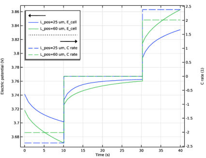
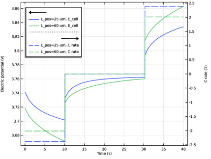
In the Settings window for Global, click Replace Expression in the upper-right corner of the y-Axis Data section. From the menu, choose Component 1 (comp1) > Definitions > Variables > C_rate - C rate - 1.
|
|
3
|
Click to expand the Coloring and Style section. Find the Line style subsection. From the Line list, choose Dashed.
|
|
4
|
|
1
|
|
2
|
|
3
|
Select the Show legends checkbox.
|
|
4
|
|
5
|
|
1
|
|
2
|
|
3
|
|
4
|
|
5
|
|
6
|
|
7
|
|
1
|
|
2
|
|
3
|
|
1
|
|
2
|
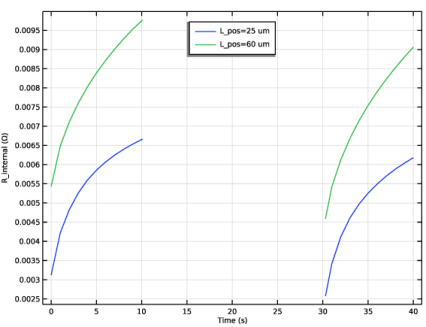
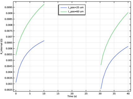
In the Settings window for Global, click Replace Expression in the upper-right corner of the y-Axis Data section. From the menu, choose Component 1 (comp1) > Definitions > Variables > R_internal - R_internal - Ω.
|
|
3
|
|
1
|
|
2
|
|
3
|
|
4
|
|
5
|
|
1
|
In the Model Builder window, under Component 1 (comp1) right-click Definitions and choose Variables.
|
|
2
|
|
3
|
Click
|
|
4
|
Browse to the model’s Application Libraries folder and double-click the file lib_internal_resistance_variables.txt.
|
|
1
|
|
2
|
|
3
|
|
1
|
|
2
|
|
3
|
|
1
|
|
2
|
|
3
|
|
1
|
|
1
|
|
2
|
|
1
|
|
2
|
|
3
|
|
4
|
|
5
|
|
6
|
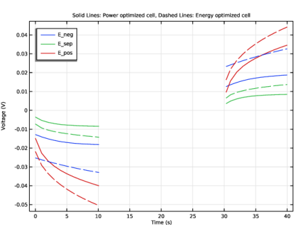
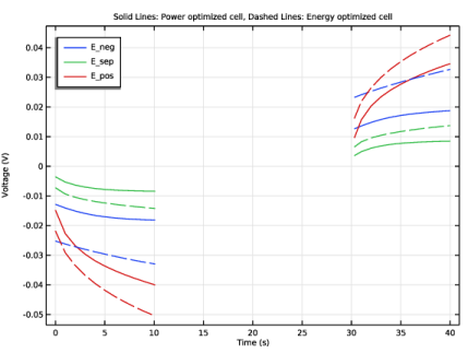
Click Add Expression in the upper-right corner of the y-Axis Data section. From the menu, choose Component 1 (comp1) > Definitions > Variables > E_neg - Voltage loss, negative - V.
|
|
7
|
Click Add Expression in the upper-right corner of the y-Axis Data section. From the menu, choose Component 1 (comp1) > Definitions > Variables > E_sep - Voltage loss, separator - V.
|
|
8
|
Click Add Expression in the upper-right corner of the y-Axis Data section. From the menu, choose Component 1 (comp1) > Definitions > Variables > E_pos - Voltage loss, positive - V.
|
|
9
|
|
10
|
Clear the Description checkbox.
|
|
11
|
Select the Expression checkbox.
|
|
1
|
|
2
|
|
3
|
|
4
|
Locate the Coloring and Style section. Find the Line style subsection. From the Line list, choose Dashed.
|
|
5
|
|
6
|
|
1
|
|
2
|
|
3
|
|
4
|
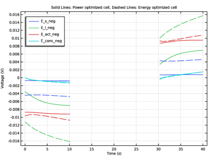
In the Title text area, type Solid Lines: Power optimized cell, Dashed Lines: Energy optimized cell.
|
|
5
|
Locate the Plot Settings section.
|
|
6
|
|
7
|
|
8
|
|
1
|
|
2
|
In the Settings window for 1D Plot Group, type Voltage Losses, Negative Electrode in the Label text field.
|
|
1
|
|
2
|
|
3
|
|
4
|
|
5
|
|
6
|
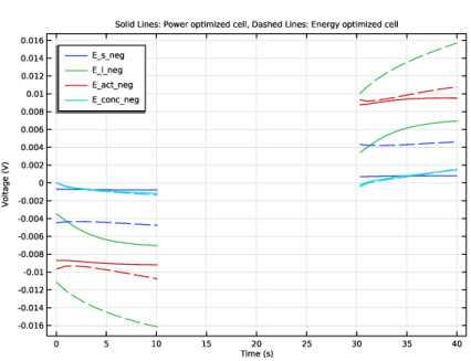
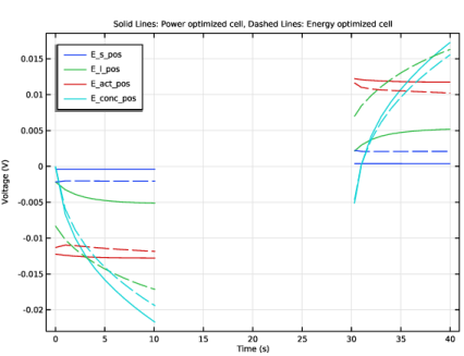
Click Replace Expression in the upper-right corner of the y-Axis Data section. From the menu, choose Component 1 (comp1) > Definitions > Variables > E_s_neg - Electrode ohmic voltage loss, negative - V.
|
|
7
|
Click Add Expression in the upper-right corner of the y-Axis Data section. From the menu, choose Component 1 (comp1) > Definitions > Variables > E_l_neg - Electrolyte ohmic voltage loss, negative - V.
|
|
8
|
Click Add Expression in the upper-right corner of the y-Axis Data section. From the menu, choose Component 1 (comp1) > Definitions > Variables > E_act_neg - Electrode activation voltage loss, negative - V.
|
|
9
|
Click Add Expression in the upper-right corner of the y-Axis Data section. From the menu, choose Component 1 (comp1) > Definitions > Variables > E_conc_neg - Concentration voltage loss, negative - V.
|
|
10
|
|
11
|
|
12
|
Clear the Description checkbox.
|
|
13
|
Select the Expression checkbox.
|
|
1
|
|
2
|
|
3
|
|
4
|
Locate the Coloring and Style section. Find the Line style subsection. From the Line list, choose Dashed.
|
|
5
|
|
6
|
|
1
|
|
2
|
|
3
|
|
4
|
|
5
|
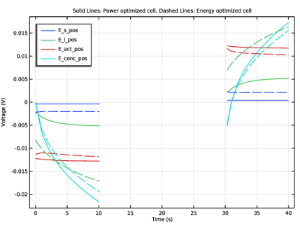
In the Title text area, type Solid Lines: Power optimized cell, Dashed Lines: Energy optimized cell.
|
|
6
|
|
7
|
|
1
|
|
2
|
In the Settings window for 1D Plot Group, type Voltage Losses, Positive Electrode in the Label text field.
|
|
1
|
In the Model Builder window, expand the Voltage Losses, Positive Electrode node, then click Global 1.
|
|
2
|
|
1
|
|
2
|
|
1
|
|
2
|