|
|
|
|
1
|
|
2
|
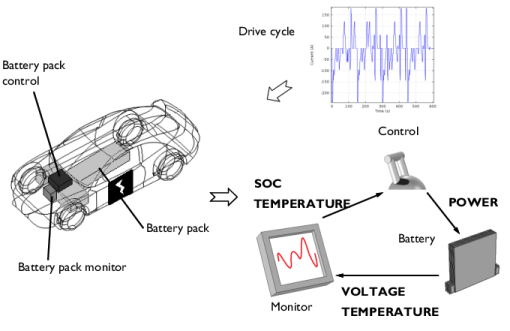
In the Application Libraries window, select Battery Design Module > Lithium-Ion Batteries, Performance > lib_base_model_1d in the tree.
|
|
3
|
Click
|
|
1
|
|
2
|
Go to the Add Physics window.
|
|
3
|
|
4
|
Click the Add to Component 1 button in the window toolbar.
|
|
5
|
|
1
|
|
2
|
|
3
|
|
4
|
|
5
|
|
6
|
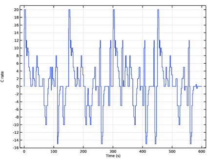
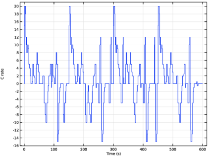
Browse to the model’s Application Libraries folder and double-click the file lib_drive_cycle_data.txt.
|
|
7
|
Locate the Auxiliary Settings section. Select the Ignore consecutive identical reinitialization expressions checkbox.
|
|
1
|
In the Model Builder window, expand the Component 1 (comp1) > Lithium-Ion Battery (liion) node, then click Electrode Current Density 1.
|
|
2
|
|
3
|
|
1
|
In the Model Builder window, expand the Porous Electrode - Negative node, then click Particle Intercalation 1.
|
|
2
|
In the Settings window for Particle Intercalation, click to expand the Particle Discretization section.
|
|
3
|
Select the Fast assembly in particle dimension checkbox.
|
|
1
|
In the Model Builder window, expand the Porous Electrode - Positive node, then click Particle Intercalation 1.
|
|
2
|
|
3
|
Select the Fast assembly in particle dimension checkbox.
|
|
1
|
|
2
|
|
1
|
|
2
|
|
3
|
|
4
|
|
5
|
|
1
|
|
2
|
|
1
|
|
2
|
|
1
|
|
2
|
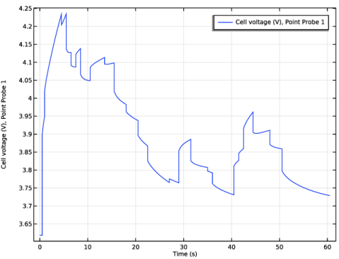
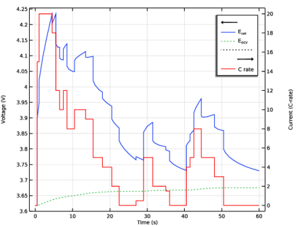
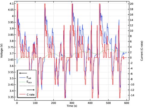
In the Settings window for Global, click Replace Expression in the upper-right corner of the y-Axis Data section. From the menu, choose Component 1 (comp1) > Definitions > E_cell - Point Probe 1 - V.
|
|
3
|
Locate the y-Axis Data section. In the table, enter the following settings:
|
|
4
|
Click Add Expression in the upper-right corner of the y-Axis Data section. From the menu, choose Component 1 (comp1) > Definitions > Variables > E_ocv_cell - Open-circuit cell voltage - V.
|
|
5
|
Click to expand the Coloring and Style section. Find the Line style subsection. From the Line list, choose Cycle.
|
|
6
|
|
1
|
|
2
|
|
4
|
|
5
|
|
1
|
|
2
|
|
3
|
|
4
|
|
5
|
|
6
|
|
7
|
|
8
|
|
1
|
|
2
|
|
3
|
|
4
|
|
1
|
|
2
|
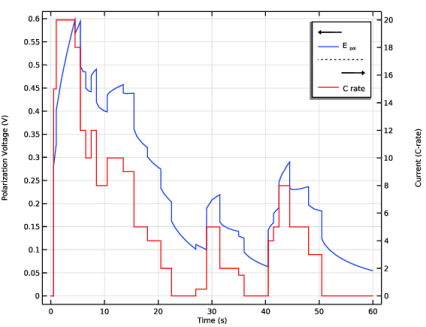
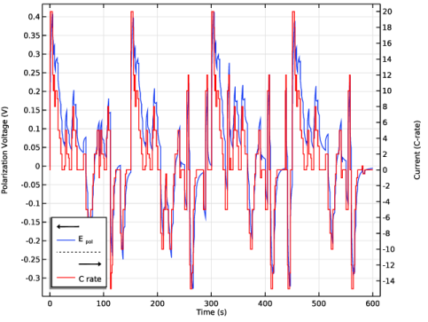
In the Settings window for Global, click Replace Expression in the upper-right corner of the y-Axis Data section. From the menu, choose Component 1 (comp1) > Definitions > Variables > E_pol_tot - Total battery cell polarization - V.
|
|
3
|
Locate the Legends section. In the table, enter the following settings:
|
|
4
|
|
1
|
|
2
|
|
1
|
|
2
|
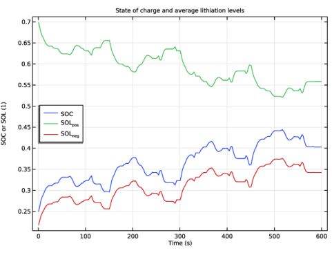
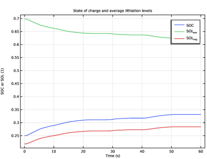
In the Settings window for Global, click Replace Expression in the upper-right corner of the y-Axis Data section. From the menu, choose Component 1 (comp1) > Definitions > Variables > soc_cell - Battery cell state of charge - 1.
|
|
3
|
Click Add Expression in the upper-right corner of the y-Axis Data section. From the menu, choose Component 1 (comp1) > Definitions > Variables > sol_pos - Degree of lithiation, positive - 1.
|
|
4
|
Click Add Expression in the upper-right corner of the y-Axis Data section. From the menu, choose Component 1 (comp1) > Definitions > Variables > sol_neg - Degree of lithiation, negative - 1.
|
|
5
|
|
6
|
|
8
|
|
1
|
|
2
|
|
3
|
|
4
|
|
5
|
Locate the Plot Settings section.
|
|
6
|
|
7
|
|
1
|
|
2
|
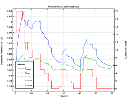
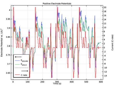
In the Settings window for 1D Plot Group, type Positive Electrode Potentials in the Label text field.
|
|
1
|
|
3
|
|
4
|
|
5
|
|
6
|
|
8
|
|
1
|
|
2
|
Select the Two y-axes checkbox.
|
|
3
|
|
4
|
Select the y-axis label checkbox. In the associated text field, type Electrode Potential vs. Li/Li<sup>+</sup>.
|
|
5
|
|
6
|
|
7
|
|
8
|
|
9
|
|
10
|
|
1
|
|
2
|
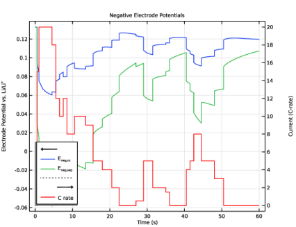
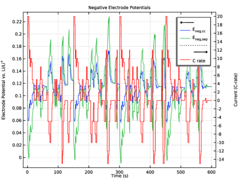
In the Settings window for 1D Plot Group, type Negative Electrode Potentials in the Label text field.
|
|
3
|
|
1
|
In the Model Builder window, expand the Negative Electrode Potentials node, then click Point Graph 1.
|
|
2
|
|
3
|
|
4
|
Click
|
|
6
|
Locate the Legends section. In the table, enter the following settings:
|
|
7
|
|
1
|
|
2
|
|
1
|
|
2
|
|
3
|
|
4
|
|
1
|
|
2
|
|
3
|
|
4
|
|
1
|
|
2
|
|
3
|
|
4
|
|
1
|
|
2
|
|
3
|
|
4
|
|
1
|
|
2
|
|
1
|
|
2
|
|
3
|
|
4
|