PDF

Newtonian Telescope Structural Analysis
Introduction
This tutorial demonstrates ray tracing through a deformed optical system. In this example, shows how a telescope is deformed under gravity and the effect this has on image quality.
The Newtonian Telescope model is used as the basis for this tutorial. First, a simple barrel and truss structure is added to the geometry, together with supports for the primary and secondary mirrors (Figure 1). The telescope can then be rotated about the azimuth axis. As a consequence, the optics will deform under the varying gravitational load (Figure 2).
Figure 1: An overview of the telescope geometry used in the Newtonian Telescope Structural Analysis tutorial. The primary and secondary mirrors are blue. The cross-section of the truss is green and the barrels are light gray. The azimuth axis (dark gray) is located at the approximate center of mass.
This tutorial first demonstrates both a single-physics simulations using the Geometrical Optics interface, followed by with analysis of the structural deformation due to gravity using the Solid Mechanics interface. Other COMSOL multiphysics models demonstrate the impact of thermal deformation due to heat transfer and surface-to-surface radiation. See, for example, the Petzval Lens STOP Analysis and Petzval Lens STOP Analysis with Surface-to-Surface Radiation tutorials. The impact of ray-heating on the optical performance is demonstrated in the Thermally Induced Focal Shift in High-Power Laser Focusing Systems tutorial.
Figure 2: The telescope structure deforms due to gravity as the inclination is changed.
Model Definition
The geometry for this model can be inserted from a predefined geometry sequence. Full step-by-step instructions can be found in Appendix — Geometry Instructions. Further details of the telescope can be found in the Newtonian Telescope tutorial.
After insertion, the geometry will look like Figure 3. After adjusting the parameter (theta) defining the telescope inclination to 45.0°, the geometry will look like Figure 4.
Because the rays will be traced in a deformed geometry, in order to avoid discretization errors, the mesh needs to be refined on the primary mirror surface. See Figure 5. Additionally, the mesh on other elements (such as the truss) is refined so that the mesh remains well structured.
The model will include two studies. In Study 1, a ray trace will be performed on the undeformed (but inclined) geometry. In Study 2 the ray trace will be performed following a computation of the structural deformation.
In each of these studies, a collimated and monochomatic bundle of rays with a hexapolar distribution is launched. The field angles correspond to the telescopes’s angle of inclination and a field 2 arcmin removed from that angle.
Figure 3: The Newtonian Telescope Structural Analysis geometry sequence.
Figure 4: The geometry sequence at an inclination of 45.0°.
Figure 5: The Newtonian Telescope Structural Analysis mesh.
Results and Discussion
The results of a ray trace through the telescope without any deformation are shown in Figure 6. The corresponding spot diagrams can be seen in Figure 7. As expected, the image quality is perfect on-axis, and subject to coma at a field angle of 2 arcminutes. This is confirmed in the aberration diagram seen in Figure 8.
After including the structural deformation, the ray trace looks like Figure 9. This figure also shows the extent to which the telescope structure is deformed under gravity. That is just over 6 μm at this inclination.
The effect on the image quality can be seen in Figure 10. These spot diagrams lie on the “best focus” image planes. This is the plane where the on-axis RMS spot size is minimized. After deformation, the on-axis spot radius is now rrms = 0.474 μm. This is also the contribution, in quadrature, to the degradation of the off-axis image quality.
As seen in the aberration diagram (Figure 11), the deformation contributes to a uncorrected defocus term.
Figure 6: A ray trace through the undeformed geometry.
Figure 7: The undeformed spot diagram.
Figure 8: The undeformed aberration diagrams. Left is on-axis and uses all Zernike terms. Right is off-axis and shows only the dominant coma terms. The scale is in waves.
Figure 9: A ray trace using the deformed geometry. The scale is exaggerated in this view.
Figure 10: The spot diagram including structural deformation.
Figure 11: The deformed aberration diagram. Both on-axis (left) and off-axis (right) diagrams show only the defocus and coma Zernike terms.
Application Library path: Ray_Optics_Module/Structural_Thermal_Optical_Performance_Analysis/newtonian_telescope_structural_analysis
Modeling Instructions
From the File menu, choose New.
New
In the New window, click  Model Wizard.
Model Wizard
1
In the Model Wizard window, click  3D.
2
In the Select Physics tree, select Optics>Ray Optics>Geometrical Optics (gop).
3
Click Add.
4
Click  Study.
5
In the Select Study tree, select Preset Studies for Selected Physics Interfaces>Ray Tracing.
6
First, a ray trace will be done on an undeformed telescope structure using only the Geometrical Optics interface. Later, the Solid Mechanics interface and associated studies will be added.
Component 1 (comp1)
1
In the Model Builder window, click Component 1 (comp1).
2
In the Settings window for Component, locate the Curved Mesh Elements section.
3
From the Geometry shape function list, choose Cubic Lagrange. The ray tracing algorithm used by the Geometrical Optics interface computes the refracted ray direction based on a discretized geometry via the underlying finite element mesh. A cubic geometry shape order introduces less discretization error compared to the default, which uses linear and quadratic polynomials.
Newtonian Telescope Structural Analysis Geometry Sequence
Insert the prepared geometry sequence from file. You can read the instructions for creating the geometry in Appendix — Geometry Instructions.
1
In the Model Builder window, under Component 1 (comp1) click Geometry 1.
2
In the Settings window for Geometry, type Newtonian Telescope Structural Analysis Geometry Sequence in the Label text field.
3
Locate the Units section. From the Length unit list, choose mm.
4
In the Geometry toolbar, click Insert Sequence and choose Insert Sequence.
5
Browse to the model’s Application Libraries folder and double-click the file newtonian_telescope_structural_analysis_geom_sequence.mph.
6
In the Insert Sequence dialog box, click OK.
7
In the Geometry toolbar, click  Build All.
8
Click the  Orthographic Projection button in the Graphics toolbar. Compare the resulting geometry to Figure 3. In the following steps, change the telescope inclination to 45 degrees.
Global Definitions
Parameters 1: Telescope Geometry
1
In the Model Builder window, under Global Definitions click Parameters 1.
2
In the Settings window for Parameters, type Parameters 1: Telescope Geometry in the Label text field. The telescope geometry parameters were added when the geometry sequence was inserted.
3
Locate the Parameters section. In the table, enter the following settings:
Parameters 2: Wavelengths and Fields
The wavelength and field parameters can be loaded from a text file.
1
In the Home toolbar, click  Parameters and choose Add>Parameters.
2
In the Settings window for Parameters, type Parameters 2: Wavelengths and Fields in the Label text field.
3
Locate the Parameters section. Click  Load from File.
4
Browse to the model’s Application Libraries folder and double-click the file newtonian_telescope_structural_analysis_parameters.txt.
Newtonian Telescope Structural Analysis Geometry Sequence
In the Home toolbar, click  Build All. Compare the resulting geometry to Figure 4.
Add Material
1
In the Home toolbar, click  Add Material to open the Add Material window.
2
Go to the Add Material window.
3
In the tree, select Built-in>Aluminum 6063-T83.
4
Click Add to Component in the window toolbar.
5
In the tree, select Built-in>Steel AISI 4340.
6
Click Add to Component in the window toolbar.
7
In the tree, select Built-in>Silica glass.
8
Click Add to Component in the window toolbar.
9
In the Home toolbar, click  Add Material to close the Add Material window.
Materials
Steel AISI 4340 (mat2)
1
In the Model Builder window, under Component 1 (comp1)>Materials click Steel AISI 4340 (mat2).
2
Silica glass (mat3)
1
In the Model Builder window, click Silica glass (mat3).
2
Geometrical Optics (gop)
1
In the Model Builder window, under Component 1 (comp1) click Geometrical Optics (gop).
2
In the Settings window for Geometrical Optics, locate the Domain Selection section.
3
Click  Clear Selection. Because this is a fully reflecting telescope, the ray tracing does not require any domains to be selected.
4
Locate the Ray Release and Propagation section. In the Maximum number of secondary rays text field, type 0.
5
Locate the Additional Variables section. Select the Compute optical path length check box. The optical path length will be used to create the aberration diagrams.
6
Select the Count reflections check box. The number of reflections (gop.Nrefl) can be used to control the behavior of physics features or during postprocessing.
Ray Properties 1
1
In the Model Builder window, under Component 1 (comp1)>Geometrical Optics (gop) click Ray Properties 1.
2
In the Settings window for Ray Properties, locate the Ray Properties section.
3
In the λ0 text field, type lam.
Release from Grid 1
In the following, hexapolar grid release features are added. The direction vectors and launch positions are defined in the Parameters node.
1
In the Physics toolbar, click  Global and choose Release from Grid.
2
In the Settings window for Release from Grid, locate the Initial Coordinates section.
3
From the Grid type list, choose Hexapolar.
4
Specify the qc vector as
5
Specify the rc vector as
6
In the Rc text field, type d_pupil/2.
7
In the Nc text field, type N_hex.
8
Locate the Ray Direction Vector section. Specify the L0 vector as
Release from Grid 2
1
Right-click Release from Grid 1 and choose Duplicate.
2
In the Settings window for Release from Grid, locate the Initial Coordinates section.
3
Specify the qc vector as
4
Specify the rc vector as
5
Locate the Ray Direction Vector section. Specify the L0 vector as
Next, define the boundary conditions. These will be specular reflection on the mirror surfaces and absorption everywhere else. Note that in order to simplify this simulation, the telescope structure is not selected to be part of the Geometrical Optics physics. Therefore, rays will pass through obstructions such as the secondary supports.
Primary Mirror
1
In the Physics toolbar, click  Boundaries and choose Mirror.
2
In the Settings window for Mirror, type Primary Mirror in the Label text field.
3
Locate the Boundary Selection section. From the Selection list, choose Mirror surface (Primary Mirror).
Secondary Mirror
1
In the Physics toolbar, click  Boundaries and choose Wall.
2
In the Settings window for Wall, type Secondary Mirror in the Label text field.
3
Locate the Boundary Selection section. From the Selection list, choose Mirror surface (Secondary Mirror).
4
Locate the Wall Condition section. From the Wall condition list, choose Specular reflection.
5
Locate the Primary Ray Condition section. From the Primary ray condition list, choose Expression.
6
In the e text field, type gop.Nrefl>0. A ray striking the secondary mirror will reflect only if it has encountered a mirror surface (that is, the Primary Mirror) previously.
7
From the Otherwise list, choose Pass through.
Primary Obstructions
1
In the Physics toolbar, click  Boundaries and choose Wall.
2
In the Settings window for Wall, type Primary Obstructions in the Label text field.
3
Locate the Wall Condition section. From the Wall condition list, choose Disappear.
4
Locate the Boundary Selection section. From the Selection list, choose Primary Obstructions.
Secondary Obstructions
1
In the Physics toolbar, click  Boundaries and choose Wall.
2
In the Settings window for Wall, type Secondary Obstructions in the Label text field.
3
Locate the Wall Condition section. From the Wall condition list, choose Disappear.
4
Locate the Boundary Selection section. From the Selection list, choose Secondary Obstructions.
Image Plane
1
In the Physics toolbar, click  Boundaries and choose Wall.
2
In the Settings window for Wall, type Image Plane in the Label text field.
3
Locate the Boundary Selection section. From the Selection list, choose Detector.
Mesh 1
The default mesh will be improved on the primary mirror surface. The extra points added around the clear aperture circumference also increase the mesh resolution near the edges of the mirror.
Size 1
1
In the Model Builder window, under Component 1 (comp1) right-click Mesh 1 and choose Size.
2
In the Settings window for Size, locate the Geometric Entity Selection section.
3
From the Geometric entity level list, choose Boundary.
4
From the Selection list, choose Mirror surface (Primary Mirror).
5
Locate the Element Size section. From the Predefined list, choose Extremely fine.
The mesh on the telescope truss (and some other surfaces) should be slightly refined.
Size 2
1
In the Model Builder window, right-click Mesh 1 and choose Size.
2
In the Settings window for Size, locate the Geometric Entity Selection section.
3
From the Geometric entity level list, choose Domain.
4
From the Selection list, choose Telescope Truss Union.
5
6
Locate the Element Size section. From the Predefined list, choose Fine.
Size 3
1
Right-click Mesh 1 and choose Size.
2
In the Settings window for Size, locate the Geometric Entity Selection section.
3
From the Geometric entity level list, choose Boundary.
4
5
Locate the Element Size section. From the Predefined list, choose Fine.
Free Tetrahedral 1
1
In the Mesh toolbar, click  Free Tetrahedral.
2
In the Settings window for Free Tetrahedral, click  Build All. Compare the resulting mesh to Figure 5.
Study 1
Now, perform the ray trace on the undeformed geometry.
Step 1: Ray Tracing
1
In the Model Builder window, under Study 1 click Step 1: Ray Tracing.
2
In the Settings window for Ray Tracing, locate the Study Settings section.
3
From the Time-step specification list, choose Specify maximum path length.
4
From the Length unit list, choose mm.
5
In the Lengths text field, type 0 2.10*f. The maximum path length is slightly greater than twice the focal length of the telescope. This ensures that all rays reach the focal plane.
6
In the Home toolbar, click  Compute.
Results
Ray Diagram - Undeformed
In the following steps, we first modify the default ray trajectories plot and then create a spot diagram.
1
In the Settings window for 3D Plot Group, type Ray Diagram - Undeformed in the Label text field.
2
Locate the Color Legend section. Select the Show units check box.
3
In the Model Builder window, expand the Ray Diagram - Undeformed node.
Color Expression 1
1
In the Model Builder window, expand the Results>Ray Diagram - Undeformed>Ray Trajectories 1 node, then click Color Expression 1.
2
In the Settings window for Color Expression, locate the Expression section.
3
In the Expression text field, type at('last',gop.rrel). This colors the ray according to their radial distance of the centroid of each release feature on the image plane.
4
In the Unit field, type um.
5
In the Ray Diagram - Undeformed toolbar, click  Plot.
6
Click the  Zoom Extents button in the Graphics toolbar. Compare this figure to Figure 6.
Spot Diagram - Undeformed
Now, create a spot diagram.
1
In the Home toolbar, click  Add Plot Group and choose 2D Plot Group.
2
In the Settings window for 2D Plot Group, type Spot Diagram - Undeformed in the Label text field.
3
Locate the Plot Settings section. Select the x-axis label check box.
4
5
Select the y-axis label check box.
6
7
Locate the Color Legend section. Select the Show units check box.
Spot Diagram 1
1
In the Spot Diagram - Undeformed toolbar, click  More Plots and choose Spot Diagram.
2
In the Settings window for Spot Diagram, click to expand the Focal Plane Orientation section.
3
From the Transverse direction list, choose User defined. This allows the orientation of the spot diagram to be controlled.
4
In the x text field, type 0.
5
In the y text field, type cos(theta).
6
In the z text field, type sin(theta).
7
Locate the Layout section. From the Origin location list, choose Average over area.
8
From the Layout list, choose Rectangular grid.
9
In the Number of columns text field, type 1.
10
Click to expand the Annotations section. Select the Show spot coordinates check box.
11
From the Coordinate system list, choose Global. Using the Global coordinate system allows the z coordinate to be displayed.
12
In the Display precision text field, type 6.
13
Select the Fit annotations to spot check box.
Color Expression 1
1
Right-click Spot Diagram 1 and choose Color Expression.
2
In the Settings window for Color Expression, locate the Expression section.
3
In the Expression text field, type at(0,gop.rrel).
4
In the Spot Diagram - Undeformed toolbar, click  Plot.
5
Click the  Zoom Extents button in the Graphics toolbar. Compare this figure to Figure 7.
Aberration Diagram - Undeformed
A wavefront aberration diagram will be created in the following steps.
1
In the Home toolbar, click  Add Plot Group and choose 2D Plot Group.
2
In the Settings window for 2D Plot Group, type Aberration Diagram - Undeformed in the Label text field.
3
Locate the Color Legend section. Select the Show units check box.
Optical Aberration 1
1
In the Aberration Diagram - Undeformed toolbar, click  More Plots and choose Optical Aberration.
2
In the Settings window for Optical Aberration, locate the Filters section.
3
Select the Filter by release feature index check box. By default, the first (on-axis) release is selected.
4
Locate the Focal Plane Orientation section. Click Create Reference Hemisphere Dataset. This will create an Intersection Point 3D dataset, with a reference hemisphere that is centered on the point that minimizes the on-axis RMS spot radius.
5
Locate the Coloring and Style section. From the Color table list, choose Dipole.
6
From the Scale list, choose Linear symmetric.
Optical Aberration 2
1
Right-click Optical Aberration 1 and choose Duplicate.
2
In the Settings window for Optical Aberration, locate the Filters section.
3
In the Filter by release feature index text field, type 2. This is the off-axis ray release.
4
Locate the Position section. In the x text field, type 2.5.
5
Locate the Zernike Polynomials section. From the Terms to include list, choose Select individual terms.
6
Select the Z(3,-1), vertical coma check box.
7
Select the Z(3,1), horizontal coma check box. As expected for a telescope with a parabolic primary mirror, the dominate off-axis aberration is coma.
8
Click to expand the Inherit Style section. From the Plot list, choose Optical Aberration 1.
9
In the Aberration Diagram - Undeformed toolbar, click  Plot.
10
Click the  Zoom Extents button in the Graphics toolbar. Compare this figure to Figure 8.
Add Physics
In the following steps, we add a structural mechanics interface so that the deformation of the telescope structure under gravity can be considered.
1
In the Home toolbar, click  Add Physics to open the Add Physics window.
2
Go to the Add Physics window.
3
In the tree, select Structural Mechanics>Solid Mechanics (solid). Next, ensure that the solid mechanics physics will not be considered in the existing study.
4
Find the Physics interfaces in study subsection. In the table, clear the Solve check box for Study 1.
5
Click Add to Component 1 in the window toolbar.
6
In the Home toolbar, click  Add Physics to close the Add Physics window.
Solid Mechanics (solid)
Gravity 1
1
Right-click Component 1 (comp1)>Solid Mechanics (solid) and choose Volume Forces>Gravity.
2
In the Settings window for Gravity, locate the Domain Selection section.
3
From the Selection list, choose All domains.
Fixed Constraint 1
1
In the Physics toolbar, click  Boundaries and choose Fixed Constraint.
2
Add Study
A new study will be used to do the combined structural and ray tracing simulation.
1
In the Home toolbar, click  Add Study to open the Add Study window.
2
Go to the Add Study window.
3
Find the Studies subsection. In the Select Study tree, select Preset Studies for Some Physics Interfaces>Stationary.
4
Find the Physics interfaces in study subsection. In the table, clear the Solve check box for Geometrical Optics (gop).
That is, ensure that the stationary study does not include the Geometrical Optics interface.
5
Click Add Study in the window toolbar.
6
In the Home toolbar, click  Add Study to close the Add Study window.
Study 2
Ray Tracing
1
In the Study toolbar, click  Study Steps and choose Time Dependent>Ray Tracing.
2
In the Settings window for Ray Tracing, locate the Study Settings section.
3
From the Time-step specification list, choose Specify maximum path length.
4
From the Length unit list, choose mm.
5
In the Lengths text field, type 0 2.10*f.
6
Select the Include geometric nonlinearity check box. Geometric nonlinearities must be included otherwise the ray trace will not be performed on the deformed telescope geometry.
7
Locate the Physics and Variables Selection section. In the table, clear the Solve for check box for Solid Mechanics (solid).
The ray tracing study should not include the Solid Mechanics interface.
Next, modify the ray tracing study to disable the image plane. This allows the Intersection Point 3D datasets used by the spot and aberration diagrams to be computed automatically.
8
Select the Modify model configuration for study step check box.
9
In the tree, select Component 1 (Comp1)>Geometrical Optics (Gop)>Image Plane.
10
11
In the Study toolbar, click  Compute.
Results
Ray Diagram - Deformed
In the following steps ray and spot diagrams are created which show the results of a ray trace through the deformed telescope geometry. An aberration diagram is also created.
1
In the Settings window for 3D Plot Group, type Ray Diagram - Deformed in the Label text field.
2
Locate the Color Legend section. Select the Show units check box.
3
In the Model Builder window, expand the Ray Diagram - Deformed node.
Color Expression 1
1
In the Model Builder window, expand the Results>Ray Diagram - Deformed>Ray Trajectories 1 node, then click Color Expression 1.
2
In the Settings window for Color Expression, locate the Coloring and Style section.
3
Clear the Color legend check box.
Surface 1
1
In the Model Builder window, right-click Ray Diagram - Deformed and choose Surface.
2
In the Settings window for Surface, locate the Expression section.
3
In the Expression text field, type solid.disp.
4
Locate the Coloring and Style section. From the Color table list, choose HeatCamera.
5
From the Color table transformation list, choose Reverse.
6
Locate the Expression section. In the Unit field, type um.
Deformation 1
Right-click Surface 1 and choose Deformation.
Transparency 1
1
In the Model Builder window, right-click Surface 1 and choose Transparency.
2
In the Ray Diagram - Deformed toolbar, click  Plot.
3
Click the  Zoom Extents button in the Graphics toolbar. Compare the result to Figure 9.
Two additional plots are created by default. The plots below show the von Mises stress and the load within the telescope volume.
Stress (solid)
1
In the Model Builder window, under Results click Stress (solid).
2
In the Stress (solid) toolbar, click  Plot.
Volume Loads (solid)
1
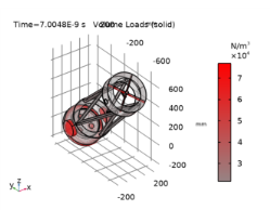
In the Model Builder window, expand the Applied Loads (solid) node, then click Volume Loads (solid).
2
In the Volume Loads (solid) toolbar, click  Plot.
Spot Diagram - Undeformed
The existing undeformed spot diagram can be used to create a new spot diagram.
Spot Diagram - Deformed
1
In the Model Builder window, right-click Spot Diagram - Undeformed and choose Duplicate.
2
In the Settings window for 2D Plot Group, type Spot Diagram - Deformed in the Label text field.
3
Locate the Data section. From the Dataset list, choose Ray 2. This dataset was created when Study 2 was run. It is necessary to use this dataset when using the Automatic Focal Plane Calculation below.
Spot Diagram 1
1
In the Model Builder window, expand the Spot Diagram - Deformed node, then click Spot Diagram 1.
2
In the Settings window for Spot Diagram, locate the Filters section.
3
Select the Filter by release feature index check box.
4
Locate the Focal Plane Orientation section. Click Create Focal Plane Dataset. This generates an Intersection Point 3D dataset that minimizes the RMS radius of the first ray release. The resulting point and normal values define the focal plane.
5
Locate the Filters section. Clear the Filter by release feature index check box. The intersection of all ray releases with the focal plane will now be shown.
6
In the Spot Diagram - Deformed toolbar, click  Plot.
7
Click the  Zoom Extents button in the Graphics toolbar. Compare this figure to Figure 10.
Aberration Diagram - Deformed
Finally, create a wavefront aberration diagram for the deformed ray trace.
1
In the Home toolbar, click  Add Plot Group and choose 2D Plot Group.
2
In the Settings window for 2D Plot Group, type Aberration Diagram - Deformed in the Label text field.
3
Locate the Color Legend section. Select the Show units check box.
4
Locate the Data section. From the Dataset list, choose Ray 2.
Optical Aberration 1
1
In the Aberration Diagram - Deformed toolbar, click  More Plots and choose Optical Aberration.
2
In the Settings window for Optical Aberration, locate the Filters section.
3
Select the Filter by release feature index check box.
4
Locate the Focal Plane Orientation section. Click Create Reference Hemisphere Dataset. Similar to the spot diagram, this generates an Intersection Point 3D dataset that is centered on the plane that minimizes the RMS radius of the first ray release. The reference hemisphere center and axis direction should be identical to the point and normal values in Intersection Point 3D 1 which also define the focal plane.
5
Locate the Zernike Polynomials section. From the Terms to include list, choose Select individual terms.
6
Select the Z(2,0), defocus check box.
7
Select the Z(3,-1), vertical coma check box.
8
Select the Z(3,1), horizontal coma check box. In this diagram, the defocus term now dominates.
9
Locate the Coloring and Style section. From the Color table list, choose Dipole.
10
From the Scale list, choose Linear symmetric.
Optical Aberration 2
1
Right-click Optical Aberration 1 and choose Duplicate.
2
In the Settings window for Optical Aberration, locate the Filters section.
3
In the Filter by release feature index text field, type 2. This is the off-axis ray release.
4
Locate the Position section. In the x text field, type 2.5.
5
Locate the Inherit Style section. From the Plot list, choose Optical Aberration 1.
6
In the Aberration Diagram - Deformed toolbar, click  Plot.
7
Click the  Zoom Extents button in the Graphics toolbar. Compare this figure to Figure 11.
Appendix — Geometry Instructions
From the File menu, choose New.
New
In the New window, click  Model Wizard.
Model Wizard
1
In the Model Wizard window, click  3D.
2
Newtonian Telescope Structural Analysis Geometry Sequence
1
In the Model Builder window, under Component 1 (comp1) click Geometry 1.
2
In the Settings window for Geometry, type Newtonian Telescope Structural Analysis Geometry Sequence in the Label text field.
3
Locate the Units section. From the Length unit list, choose mm.
Global Definitions
Load the model parameters from a text file.
Parameters 1
1
In the Model Builder window, under Global Definitions click Parameters 1.
2
In the Settings window for Parameters, locate the Parameters section.
3
Click  Load from File.
4
Browse to the model’s Application Libraries folder and double-click the file newtonian_telescope_structural_analysis_geom_sequence_parameters.txt.
Newtonian Telescope Structural Analysis Geometry Sequence
Center of Mass
1
In the Geometry toolbar, click  Work Plane.
2
In the Settings window for Work Plane, type Center of Mass in the Label text field.
3
Locate the Plane Definition section. From the Plane type list, choose Transformed.
4
Find the Rotation subsection. From the Axis type list, choose xw-axis.
5
In the Rotation angle text field, type theta.
Insert the Newtonian Telescope geometry sequence from file. For detailed instructions on creating this geometry see the appendix.
6
In the Geometry toolbar, click Insert Sequence and choose Insert Sequence.
7
Browse to the model’s Application Libraries folder and double-click the file newtonian_telescope_structural_analysis_newtonian_telescope_geom_sequence.mph.
Primary Mirror (pi1)
1
In the Model Builder window, click Primary Mirror (pi1).
2
In the Settings window for Part Instance, locate the Input Parameters section.
3
4
Locate the Position and Orientation of Output section. Find the Coordinate system to match subsection. From the Work plane list, choose Center of Mass (wp1).
5
Find the Displacement subsection. In the xw text field, type -cx.
6
In the yw text field, type -cy.
7
In the zw text field, type -cz. These are the approximate coordinates of the center of mass defined in the Parameters node.
8
Find the Rotation subsection. In the Rotation angle text field, type 180. Rotate the telescope by 180 degrees about the z-axis (optical axis).
9
Click to expand the Point Selections section. In the table, select the Keep check box for Mirror vertex.
10
Click  Build All Objects.
11
Click the  Orthographic Projection button in the Graphics toolbar.
12
Click the  Zoom Extents button in the Graphics toolbar.
Global Definitions
In the following steps a simple telescope tube part is created.
Telescope Tube
1
In the Model Builder window, under Global Definitions right-click Geometry Parts and choose 3D Part.
2
In the Settings window for Part, type Telescope Tube in the Label text field.
3
Locate the Input Parameters section. In the table, enter the following settings:
Upper Ring Base
1
In the Geometry toolbar, click  Parts and choose Circular Planar Annulus.
2
In the Settings window for Part Instance, type Upper Ring Base in the Label text field.
3
Locate the Input Parameters section. In the table, enter the following settings:
Upper Ring
1
In the Geometry toolbar, click  Extrude.
2
In the Settings window for Extrude, type Upper Ring in the Label text field.
3
On the object pi1, select Boundary 1 only.
4
Locate the Distances section. In the table, enter the following settings:
Lower Ring Base
1
In the Geometry toolbar, click  Parts and choose Circular Planar Annulus.
2
In the Settings window for Part Instance, type Lower Ring Base in the Label text field.
3
Locate the Input Parameters section. In the table, enter the following settings:
4
Locate the Position and Orientation of Output section. Find the Coordinate system to match subsection. From the Take work plane from list, choose Upper Ring Base (pi1).
5
From the Work plane list, choose Surface (wp1).
6
Find the Displacement subsection. In the zw text field, type L.
Lower Ring
1
In the Geometry toolbar, click  Extrude.
2
In the Settings window for Extrude, type Lower Ring in the Label text field.
3
On the object pi2, select Boundary 1 only.
4
Locate the Distances section. In the table, enter the following settings:
5
Select the Reverse direction check box.
Wall Base
1
In the Geometry toolbar, click  Parts and choose Circular Planar Annulus.
2
In the Settings window for Part Instance, type Wall Base in the Label text field.
3
Locate the Input Parameters section. In the table, enter the following settings:
4
Locate the Position and Orientation of Output section. Find the Coordinate system to match subsection. From the Take work plane from list, choose Upper Ring Base (pi1).
5
From the Work plane list, choose Surface (wp1).
6
Find the Displacement subsection. In the zw text field, type T1.
Wall
1
In the Geometry toolbar, click  Extrude.
2
In the Settings window for Extrude, type Wall in the Label text field.
3
On the object pi3, select Boundary 1 only.
4
Locate the Distances section. From the Specify list, choose Vertices to extrude to.
5
On the object ext2, select Point 1 only.
6
In the Geometry toolbar, click  Build All.
Newtonian Telescope Structural Analysis Geometry Sequence
Now, use this part to create the telescope structure.
Lower Mount
1
In the Geometry toolbar, click  Parts and choose Telescope Tube.
2
In the Settings window for Part Instance, type Lower Mount in the Label text field.
3
Locate the Input Parameters section. In the table, enter the following settings:
4
Locate the Position and Orientation of Output section. Find the Coordinate system to match subsection. From the Take work plane from list, choose Primary Mirror (pi1).
5
From the Work plane list, choose Mirror rear (wp2).
6
Find the Displacement subsection. In the zw text field, type -185.0[mm].
Primary Mirror Support 1
1
In the Geometry toolbar, click  Cylinder. This cylinder will be used to construct a simple mirror support.
2
In the Settings window for Cylinder, type Primary Mirror Support 1 in the Label text field.
3
Locate the Coordinate System section. From the Take work plane from list, choose Primary Mirror (pi1).
4
From the Work plane list, choose Mirror rear (wp2).
5
Locate the Size and Shape section. In the Radius text field, type 25.
6
In the Height text field, type 10.
7
Click  Build Selected.
8
Locate the Position section. In the yw text field, type 75.
Primary Mirror Support 1-3
1
In the Geometry toolbar, click  Transforms and choose Rotate.
2
In the Settings window for Rotate, type Primary Mirror Support 1-3 in the Label text field.
3
4
Locate the Rotation section. In the Angle text field, type 0 120 240.
5
Locate the Coordinate System section. From the Take work plane from list, choose Primary Mirror (pi1).
Altitude Axis
1
In the Geometry toolbar, click  Cylinder. This cylinder will be used to create the telescope altitude axis.
2
In the Settings window for Cylinder, type Altitude Axis in the Label text field.
3
Locate the Size and Shape section. In the Radius text field, type 75.
4
In the Height text field, type 450.
5
Locate the Position section. In the x text field, type -225.
6
In the z text field, type -cz.
7
Locate the Axis section. From the Axis type list, choose x-axis.
8
Locate the Coordinate System section. From the Take work plane from list, choose Primary Mirror (pi1).
9
From the Work plane list, choose Mirror vertex intersection (wp1).
Altitude Axis Partition Domains
1
In the Geometry toolbar, click  Booleans and Partitions and choose Partition Domains.
2
In the Settings window for Partition Domains, type Altitude Axis Partition Domains in the Label text field.
3
On the object cyl2, select Domain 1 only.
4
Locate the Partition Domains section. From the Partition with list, choose Faces.
5
On the object pi5(3), select Boundaries 1, 2, 7, and 10 only.
Altitude Axis Delete Entities
1
In the Model Builder window, right-click Newtonian Telescope Structural Analysis Geometry Sequence and choose Delete Entities.
2
In the Settings window for Delete Entities, type Altitude Axis Delete Entities in the Label text field.
3
Locate the Entities or Objects to Delete section. From the Geometric entity level list, choose Domain.
4
On the object pard1, select Domain 2 only.
Upper Mount
1
In the Geometry toolbar, click  Parts and choose Telescope Tube.
2
In the Settings window for Part Instance, type Upper Mount in the Label text field.
3
Locate the Input Parameters section. In the table, enter the following settings:
4
Locate the Position and Orientation of Output section. Find the Coordinate system to match subsection. From the Take work plane from list, choose Secondary Mirror (pi2).
5
From the Work plane list, choose Reference plane (wp1).
6
Find the Displacement subsection. In the zw text field, type -40[mm].
Update the telescope secondary obstruction parameters so that the part can be used to create the secondary mirror mount.
Secondary Obstruction (pi3)
1
In the Model Builder window, click Secondary Obstruction (pi3).
2
In the Settings window for Part Instance, locate the Input Parameters section.
3
4
Locate the Position and Orientation of Output section. Find the Displacement subsection. In the xw text field, type 0.
5
In the zw text field, type 75.0[mm].
Secondary Mirror Mount
1
In the Geometry toolbar, click  Extrude.
2
In the Settings window for Extrude, type Secondary Mirror Mount in the Label text field.
3
Locate the General section. From the Extrude from list, choose Faces.
4
On the object pi3, select Boundary 1 only.
5
Locate the Distances section. From the Specify list, choose Vertices to extrude to.
6
On the object pi2, select Point 2 only.
Secondary Mirror Mount Partition Domains
1
In the Geometry toolbar, click  Booleans and Partitions and choose Partition Domains.
2
In the Settings window for Partition Domains, type Secondary Mirror Mount Partition Domains in the Label text field.
3
On the object ext1, select Domain 1 only.
4
Locate the Partition Domains section. From the Partition with list, choose Faces.
5
On the object pi2, select Boundary 3 only.
Secondary Mirror Mount Delete Entities
1
In the Model Builder window, right-click Newtonian Telescope Structural Analysis Geometry Sequence and choose Delete Entities.
2
In the Settings window for Delete Entities, type Secondary Mirror Mount Delete Entities in the Label text field.
3
Locate the Entities or Objects to Delete section. From the Geometric entity level list, choose Domain.
4
On the object pard2, select Domain 1 only.
Secondary Support 1
1
In the Geometry toolbar, click  Block.
2
In the Settings window for Block, type Secondary Support 1 in the Label text field.
3
Locate the Size and Shape section. In the Width text field, type d0_tube.
4
In the Depth text field, type 2.5[mm].
5
In the Height text field, type 30[mm].
6
Locate the Position section. From the Base list, choose Center.
7
In the z text field, type 58[mm].
8
Locate the Rotation Angle section. In the Rotation text field, type 45.
9
Locate the Coordinate System section. From the Take work plane from list, choose Secondary Mirror (pi2).
10
From the Work plane list, choose Reference plane (wp1).
Secondary Support Partition Domains
1
In the Geometry toolbar, click  Booleans and Partitions and choose Partition Domains.
2
In the Settings window for Partition Domains, type Secondary Support Partition Domains in the Label text field.
3
On the object blk1, select Domain 1 only.
4
Locate the Partition Domains section. From the Partition with list, choose Faces.
5
On the object del2, select Boundaries 1 and 10 only.
6
On the object pi6(3), select Boundaries 5 and 9 only.
Secondary Support Delete Entities
1
Right-click Newtonian Telescope Structural Analysis Geometry Sequence and choose Delete Entities.
2
In the Settings window for Delete Entities, type Secondary Support Delete Entities in the Label text field.
3
Locate the Entities or Objects to Delete section. From the Geometric entity level list, choose Domain.
4
On the object pard3, select Domains 1, 3, and 5 only.
Secondary Support 1-2
1
In the Geometry toolbar, click  Transforms and choose Rotate.
2
In the Settings window for Rotate, type Secondary Support 1-2 in the Label text field.
3
4
Locate the Rotation section. In the Angle text field, type 0 90.
5
Locate the Coordinate System section. From the Take work plane from list, choose Primary Mirror (pi1).
Image Plane Projection
1
In the Geometry toolbar, click  Cylinder.
2
In the Settings window for Cylinder, type Image Plane Projection in the Label text field.
3
Locate the Size and Shape section. In the Radius text field, type 22.5[mm].
4
In the Height text field, type 50[mm].
5
Locate the Coordinate System section. From the Take work plane from list, choose Image Plane (pi4).
Image Plane Difference
1
In the Geometry toolbar, click  Booleans and Partitions and choose Difference.
2
In the Settings window for Difference, type Image Plane Difference in the Label text field.
3
Select the object pi6(3) only.
4
Locate the Difference section. Find the Objects to subtract subsection. Click to select the  Activate Selection toggle button.
5
Truss Base
1
In the Geometry toolbar, click  Parts and choose Circular Planar Annulus.
2
In the Settings window for Part Instance, type Truss Base in the Label text field.
3
Locate the Input Parameters section. In the table, enter the following settings:
4
Locate the Position and Orientation of Output section. Find the Coordinate system to match subsection. From the Take work plane from list, choose Lower Mount (pi5).
5
Find the Displacement subsection. In the xw text field, type R_truss.
Truss 1
1
In the Geometry toolbar, click  Extrude.
2
In the Settings window for Extrude, type Truss 1 in the Label text field.
3
Locate the General section. From the Extrude from list, choose Faces.
4
On the object pi7, select Boundary 1 only.
5
Locate the Distances section. From the Specify list, choose Vertices to extrude to.
6
On the object pi6(1), select Point 15 only.
7
Click to expand the Displacements section. In the table, enter the following settings:
Work Plane 2 (wp2)
1
In the Geometry toolbar, click  Work Plane.
2
In the Settings window for Work Plane, locate the Plane Definition section.
3
From the Plane type list, choose Transformed.
4
From the Take work plane from list, choose Primary Mirror (pi1).
5
Find the Rotation subsection. From the Axis type list, choose xw-axis.
6
In the Rotation angle text field, type 90.
Work Plane 3 (wp3)
1
In the Geometry toolbar, click  Work Plane.
2
In the Settings window for Work Plane, locate the Plane Definition section.
3
From the Plane type list, choose Transformed.
4
From the Work plane to transform list, choose Work Plane 2 (wp2).
5
Find the Rotation subsection. From the Axis type list, choose yw-axis.
6
In the Rotation angle text field, type -45.
Truss Partition Domains 1
1
In the Geometry toolbar, click  Booleans and Partitions and choose Partition Domains.
2
In the Settings window for Partition Domains, type Truss Partition Domains 1 in the Label text field.
3
On the object ext2, select Domain 1 only.
4
Locate the Partition Domains section. From the Work plane list, choose Work Plane 2 (wp2).
Truss Partition Domains 2
1
In the Geometry toolbar, click  Booleans and Partitions and choose Partition Domains.
2
In the Settings window for Partition Domains, type Truss Partition Domains 2 in the Label text field.
3
On the object pard4, select Domain 2 only.
Truss Delete Entities
1
Right-click Newtonian Telescope Structural Analysis Geometry Sequence and choose Delete Entities.
2
In the Settings window for Delete Entities, type Truss Delete Entities in the Label text field.
3
Locate the Entities or Objects to Delete section. From the Geometric entity level list, choose Domain.
4
On the object pard5, select Domains 1 and 3 only.
Truss 2
1
In the Geometry toolbar, click  Transforms and choose Mirror.
2
In the Settings window for Mirror, type Truss 2 in the Label text field.
3
Locate the Input section. Select the Keep input objects check box.
4
5
Locate the Normal Vector to Plane of Reflection section. In the y text field, type 1.
6
In the z text field, type 0.
7
Locate the Coordinate System section. From the Take work plane from list, choose Primary Mirror (pi1).
Telescope Truss 1-8
1
In the Geometry toolbar, click  Transforms and choose Rotate.
2
In the Settings window for Rotate, type Telescope Truss 1-8 in the Label text field.
3
Select the objects del4 and mir1 only.
4
Locate the Rotation section. In the Angle text field, type 0 90 180 270.
5
Locate the Coordinate System section. From the Take work plane from list, choose Primary Mirror (pi1).
Telescope Truss Union
1
In the Geometry toolbar, click  Booleans and Partitions and choose Union.
2
In the Settings window for Union, type Telescope Truss Union in the Label text field.
3
Select the objects rot3(1), rot3(2), rot3(3), rot3(4), rot3(5), rot3(6), rot3(7), and rot3(8) only.
4
Locate the Union section. Clear the Keep interior boundaries check box.
5
Locate the Selections of Resulting Entities section. Select the Resulting objects selection check box.
6
From the Show in physics list, choose All levels.
7
In the Geometry toolbar, click  Build All. Compare the resulting geometry to Figure 3.