
|
|
|

|
1
|
|
2
|
|
3
|
Click Add.
|
|
4
|
Click
|
|
5
|
|
6
|
Click
|
|
1
|
|
2
|
In the Settings window for Parameters, type Parameters 1: Telescope Geometry in the Label text field. The telescope geometry parameters will be added when the geometry sequence is inserted.
|
|
1
|
|
2
|
In the Settings window for Parameters, type Parameters 2: Wavelengths and Fields in the Label text field.
|
|
3
|
|
4
|
Browse to the model’s Application Libraries folder and double-click the file newtonian_telescope_parameters.txt.
|
|
1
|
|
2
|
|
3
|
From the Geometry shape function list, choose Cubic Lagrange. The ray tracing algorithm used by the Geometrical Optics interface computes the refracted ray direction based on a discretized geometry via the underlying finite element mesh. A cubic geometry shape order introduces less discretization error compared to the default, which uses linear and quadratic polynomials.
|
|
1
|
|
2
|
|
3
|
|
4
|
|
5
|
Browse to the model’s Application Libraries folder and double-click the file newtonian_telescope_geom_sequence.mph.
|
|
6
|
|
7
|
|
8
|
|
1
|
|
2
|
|
3
|
|
4
|
Select the Use geometry normals for ray-boundary interactions check box. In this simulation, the geometry normals are used to apply the boundary conditions for specular reflection. This is appropriate for the highest accuracy ray traces in single-physics simulations, where the geometry is not deformed.
|
|
5
|
Locate the Additional Variables section. Select the Count reflections check box. The number of reflections (gop.Nrefl) can be used to control the behavior of physics features or during postprocessing.
|
|
1
|
In the Model Builder window, under Component 1 (comp1)>Geometrical Optics (gop) click Medium Properties 1.
|
|
2
|
|
3
|
From the n list, choose User defined. The rays only propagate in the empty space around the mirrors, not through the mirrors themselves, so the refractive index in the domains can be given an arbitrary value like n=1.
|
|
1
|
|
2
|
|
3
|
|
1
|
|
2
|
|
3
|
|
4
|
|
5
|
|
6
|
|
7
|
|
8
|
|
1
|
|
2
|
|
3
|
|
4
|
|
1
|
|
2
|
|
3
|
|
4
|
|
1
|
|
2
|
|
3
|
Locate the Boundary Selection section. From the Selection list, choose Mirror surface (Primary Mirror).
|
|
1
|
|
2
|
|
3
|
Locate the Boundary Selection section. From the Selection list, choose Mirror surface (Secondary Mirror).
|
|
4
|
|
5
|
|
6
|
|
7
|
|
1
|
|
2
|
|
3
|
|
4
|
|
1
|
|
2
|
|
3
|
|
4
|
|
1
|
|
2
|
|
3
|
|
1
|
|
2
|
|
3
|
|
4
|
|
5
|
In the Lengths text field, type 0 2.25*f. The maximum path length is slightly greater than twice the focal length of the telescope. This ensures that all rays reach the focal plane.
|
|
6
|
|
1
|
|
2
|
|
3
|
|
1
|
In the Model Builder window, expand the Results>Ray Diagram>Ray Trajectories 1 node, then click Color Expression 1.
|
|
2
|
|
3
|
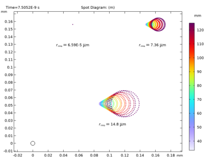
In the Expression text field, type at('last',gop.rrel). This expression gives the radial distance from the centroid of the spot on the image plane generated by each release feature.
|
|
4
|
|
5
|
|
1
|
|
2
|
|
3
|
|
4
|
In the Logical expression for inclusion text field, type gop.Nrefl>0. This will render only the rays after reflection from the primary mirror.
|
|
1
|
In the Model Builder window, under Results>Ray Diagram right-click Ray Trajectories 1 and choose Duplicate.
|
|
2
|
|
3
|
|
1
|
|
2
|
|
3
|
|
1
|
|
2
|
|
3
|
|
1
|
|
2
|
|
3
|
|
4
|
|
5
|
|
1
|
|
2
|
|
3
|
|
1
|
|
2
|
|
3
|
|
4
|
|
1
|
|
2
|
|
3
|
In the Expression text field, type at(0,gop.rrel). This is the radial coordinate relative to the centroid at the entrance pupil for each ray release.
|
|
4
|
|
5
|
|
1
|
|
2
|
Click
|
|
1
|
|
2
|
In the Settings window for Geometry, type Newtonian Telescope Geometry Sequence in the Label text field.
|
|
3
|
|
1
|
|
2
|
|
3
|
|
4
|
Browse to the model’s Application Libraries folder and double-click the file newtonian_telescope_geom_sequence_parameters.txt.
|
|
1
|
|
2
|
|
3
|
In the Part Libraries window, select Ray Optics Module>3D>Mirrors>conic_mirror_on_axis_3d in the tree.
|
|
4
|
|
5
|
In the Select Part Variant dialog box, select Specify clear aperture diameter in the Select part variant list.
|
|
6
|
Click OK.
|
|
1
|
In the Model Builder window, under Component 1 (comp1)>Newtonian Telescope Geometry Sequence click Conic Mirror On Axis 3D 1 (pi1).
|
|
2
|
|
3
|
|
4
|
|
5
|
|
6
|
Click OK. This selection, and those that follow will be used to apply boundary conditions later in the model setup.
|
|
7
|
|
8
|
|
9
|
|
10
|
Click OK.
|
|
11
|
|
12
|
|
13
|
|
14
|
Click OK.
|
|
15
|
|
1
|
|
2
|
|
3
|
In the Part Libraries window, select Ray Optics Module>3D>Mirrors>elliptical_planar_mirror_3d in the tree.
|
|
4
|
|
5
|
In the Select Part Variant dialog box, select Specify mirror angle and minor axis diameter in the Select part variant list.
|
|
6
|
Click OK.
|
|
1
|
In the Model Builder window, under Component 1 (comp1)>Newtonian Telescope Geometry Sequence click Elliptical Planar Mirror 3D 1 (pi2).
|
|
2
|
|
3
|
|
4
|
Locate the Position and Orientation of Output section. Find the Coordinate system to match subsection. From the Take work plane from list, choose Primary Mirror (pi1).
|
|
5
|
|
6
|
Find the Displacement subsection. In the zw text field, type -(f-f_image). Note that the work plane that intersects the primary mirror vertex is defined prior to a reflection. Therefore, the relative position of the secondary mirror is negative.
|
|
7
|
|
1
|
|
2
|
|
3
|
In the Part Libraries window, select Ray Optics Module>3D>Apertures and Obstructions>circular_planar_annulus in the tree.
|
|
4
|
|
1
|
In the Model Builder window, under Component 1 (comp1)>Newtonian Telescope Geometry Sequence click Circular Planar Annulus 1 (pi3).
|
|
2
|
|
3
|
|
4
|
Locate the Position and Orientation of Output section. Find the Coordinate system to match subsection. From the Take work plane from list, choose Secondary Mirror (pi2).
|
|
5
|
|
6
|
|
7
|
|
8
|
|
1
|
|
2
|
|
3
|
|
4
|
Locate the Position and Orientation of Output section. Find the Coordinate system to match subsection. From the Take work plane from list, choose Secondary Mirror (pi2).
|
|
5
|
|
6
|
|
7
|
|
8
|
|
9
|
|
10
|