
|
|
|

|
1
|
|
2
|
|
3
|
Click Add. This will add interfaces for Geometrical Optics and Heat Transfer in Solids and a Ray Heat Source multiphysics coupling.
|
|
4
|
|
5
|
Click Add.
|
|
6
|
Click
|
|
7
|
In the Select Study tree, select Preset Studies for Selected Physics Interfaces>Geometrical Optics>Bidirectionally Coupled Ray Tracing.
|
|
8
|
Click
|
|
1
|
|
2
|
|
3
|
|
4
|
Browse to the model’s Application Libraries folder and double-click the file thermally_induced_focal_shift_parameters.txt.
|
|
1
|
|
2
|
|
3
|
From the Geometry shape function list, choose Cubic Lagrange. The ray tracing algorithm used by the Geometrical Optics interface computes the refracted ray direction based on a discretized geometry via the underlying finite element mesh. A cubic geometry shape order usually introduces less discretization error compared to the default, which uses linear and quadratic polynomials.
|
|
1
|
|
2
|
|
3
|
|
1
|
|
2
|
In the Part Libraries window, select Ray Optics Module>3D>Spherical Lenses>spherical_lens_3d in the tree.
|
|
3
|
|
4
|
In the Select Part Variant dialog box, select Specify clear aperture diameter in the Select part variant list.
|
|
5
|
Click OK.
|
|
1
|
|
2
|
|
4
|
Locate the Position and Orientation of Output section. Find the Displacement subsection. In the yw text field, type -dis/2.
|
|
5
|
|
6
|
|
7
|
|
8
|
Click OK.
|
|
1
|
|
2
|
|
3
|
|
4
|
|
5
|
|
6
|
|
1
|
|
2
|
Select the object cyl1 only.
|
|
3
|
|
4
|
|
5
|
|
6
|
|
1
|
|
2
|
Select the object cyl1 only.
|
|
3
|
|
4
|
|
1
|
|
2
|
|
3
|
|
4
|
Select the object pi1 only.
|
|
5
|
|
6
|
|
1
|
|
2
|
Select the object par1 only.
|
|
3
|
|
4
|
|
1
|
|
2
|
|
3
|
|
4
|
On the object uni1, select Boundaries 1–4, 7, and 8 only.
|
|
1
|
|
2
|
|
3
|
|
4
|
|
5
|
|
6
|
Click OK.
|
|
1
|
|
2
|
Select the object uni1 only.
|
|
3
|
|
4
|
|
5
|
|
6
|
|
7
|
|
1
|
|
2
|
|
3
|
In the Part Libraries window, select Ray Optics Module>3D>Apertures and Obstructions>circular_planar_annulus in the tree.
|
|
4
|
|
1
|
In the Model Builder window, under Component 1 (comp1)>Geometry 1 click Circular Planar Annulus 1 (pi2).
|
|
2
|
|
3
|
|
4
|
Locate the Position and Orientation of Output section. Find the Displacement subsection. In the yw text field, type dis/2+Tc+bfl.
|
|
5
|
|
6
|
|
7
|
|
1
|
In the Model Builder window, under Component 1 (comp1) right-click Definitions and choose Variables.
|
|
2
|
|
3
|
|
4
|
Browse to the model’s Application Libraries folder and double-click the file thermally_induced_focal_shift_variables.txt.
|
|
1
|
|
2
|
|
3
|
In the Maximum number of secondary rays text field, type 0. Since an anti-reflective coating will be applied to the lens surfaces, it is not necessary to allocate secondary rays to model the reflection of stray light by the lens system.
|
|
1
|
In the Model Builder window, under Component 1 (comp1)>Geometrical Optics (gop) click Material Discontinuity 1.
|
|
2
|
|
3
|
|
1
|
|
2
|
|
3
|
|
1
|
|
2
|
|
3
|
|
4
|
|
5
|
|
6
|
In the Nθ text field, type 18. A conical hexapolar distribution with 18 rings will release 1027 rays.
|
|
7
|
Specify the r vector as
|
|
8
|
|
9
|
|
1
|
|
2
|
|
3
|
|
4
|
Locate the Wall Condition section. From the Wall condition list, choose Pass through. Allow the rays to pass through the target so that the location of the best focus planes can be computed.
|
|
1
|
In the Physics toolbar, click
|
|
2
|
|
3
|
|
4
|
|
5
|
In the Dependent variable quantity table, enter the following settings:
|
|
1
|
|
2
|
|
3
|
From the Temperature list, choose Cubic Lagrange. A cubic shape order usually introduces less discretization error compared to the default.
|
|
1
|
|
2
|
|
3
|
|
4
|
|
5
|
|
6
|
|
1
|
|
2
|
|
3
|
From the Displacement field list, choose Cubic Lagrange. The ray tracing will now be done on a deformed mesh. In order to reduce the discretization error a cubic shape order should be used.
|
|
1
|
|
2
|
|
3
|
|
1
|
|
2
|
Click in the Graphics window and then press Ctrl+A to select both domains.
|
|
3
|
|
4
|
|
1
|
|
2
|
|
3
|
Find the Expression for remaining selection subsection. In the Volume reference temperature text field, type T0.
|
|
1
|
|
2
|
|
3
|
|
4
|
|
5
|
|
1
|
|
1
|
|
2
|
|
3
|
|
4
|
|
5
|
|
6
|
|
7
|
|
1
|
|
2
|
|
3
|
|
1
|
|
2
|
|
3
|
Click the Custom button.
|
|
4
|
|
1
|
|
2
|
|
3
|
|
1
|
|
2
|
|
3
|
Click the Custom button.
|
|
4
|
|
1
|
|
2
|
|
1
|
|
2
|
|
3
|
|
4
|
|
5
|
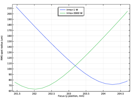
In the Lengths text field, type 0 400 range(414,0.2,419). By using smaller optical path length intervals in the vicinity of the focal plane it will be easier to observe where the mean radial displacement of the rays reaches a minimum.
|
|
6
|
Select the Include geometric nonlinearity check box. When this check box is selected, rays are traced through the deformed geometry in which thermal expansion has been taken into account. If this check box is cleared, the temperature dependence of the refractive index still affects the ray trajectories, but the thermal expansion has no effect.
|
|
7
|
|
1
|
|
2
|
|
3
|
Click
|
|
1
|
|
2
|
|
3
|
In the Model Builder window, expand the Study 1>Solver Configurations>Solution 1 (sol1)>Dependent Variables 2 node, then click Displacement field (comp1.u).
|
|
4
|
|
5
|
|
6
|
|
1
|
|
2
|
|
3
|
|
4
|
From the Selection list, choose Clear Apertures. This will be used to limit the results of some plots to the convex surfaces of the two lenses.
|
|
1
|
|
2
|
|
3
|
|
4
|
|
5
|
|
1
|
In the Model Builder window, expand the Results>Ray Trajectories (gop)>Ray Trajectories 1 node, then click Color Expression 1.
|
|
2
|
|
3
|
|
4
|
|
5
|
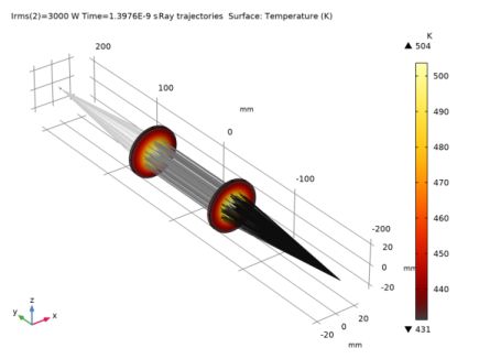
Click to expand the Range section. Locate the Coloring and Style section. From the Color table list, choose GrayPrint.
|
|
6
|
|
1
|
|
2
|
|
3
|
|
4
|
|
1
|
|
2
|
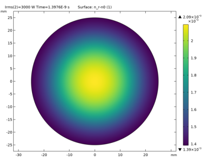
In the Settings window for Surface, click Replace Expression in the upper-right corner of the Expression section. From the menu, choose Component 1 (comp1)>Heat Transfer in Solids>Temperature>T - Temperature - K.
|
|
3
|
|
4
|
|
1
|
|
2
|
|
3
|
|
4
|
|
5
|
|
1
|
|
2
|
|
3
|
|
4
|
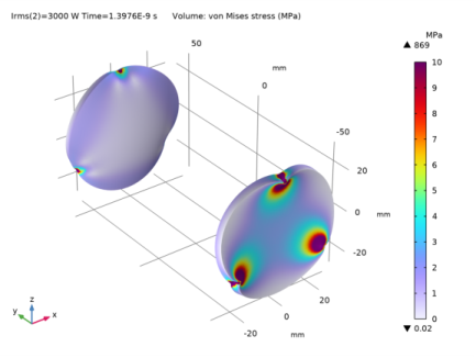
Click to expand the Range section. Specify a manual color range to make the von Mises stress easier to see.
|
|
5
|
|
6
|
|
7
|
|
8
|
|
1
|
|
2
|
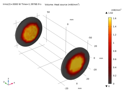
In the Settings window for 3D Plot Group, type Deposited Ray Power (lenses) in the Label text field.
|
|
3
|
|
4
|
|
5
|
|
6
|
|
1
|
|
2
|
In the Settings window for Volume, click Replace Expression in the upper-right corner of the Expression section. From the menu, choose Component 1 (comp1)>Heating and losses>rhs1.Qsrc - Heat source - W/m³.
|
|
3
|
|
4
|
|
5
|
|
6
|
|
7
|
|
8
|
|
1
|
|
2
|
|
3
|
|
4
|
|
1
|
|
2
|
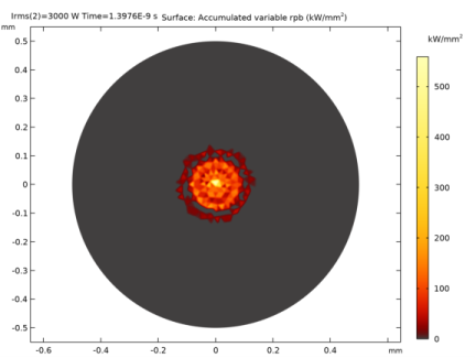
In the Settings window for 2D Plot Group, type Deposited Ray Power (target) in the Label text field.
|
|
3
|
|
4
|
|
5
|
|
1
|
|
2
|
In the Settings window for Surface, click Replace Expression in the upper-right corner of the Expression section. From the menu, choose Component 1 (comp1)>Geometrical Optics>Accumulated variables>Accumulated variable comp1.gop.wall1.bacc1.rpb>gop.wall1.bacc1.rpb - Accumulated variable rpb - W/m².
|
|
3
|
|
4
|
|
5
|
|
6
|
|
1
|
|
2
|
|
3
|
|
1
|
|
2
|
|
3
|
|
4
|
|
1
|
|
2
|
|
3
|
|
4
|
Click to expand the Title section. Locate the Coloring and Style section. From the Color table list, choose Viridis.
|
|
5
|
|
1
|
|
2
|
|
3
|
|
4
|
|
5
|
Click
|
|
6
|
|
7
|
|
8
|
Click Replace.
|
|
1
|
|
2
|
|
4
|
|
5
|
|
6
|
In the Expression text field, type gop.qavey. This is the average position along the optical axis at each time step.
|
|
1
|
|
2
|
|
3
|
|
4
|
|
5
|
|
6
|
|
7
|
|
8
|
|
1
|
|
2
|
|
3
|
|
1
|
|
2
|
|
3
|
|
1
|
|
2
|
|
3
|
|
4
|
|
1
|
|
2
|
|
3
|
|
4
|
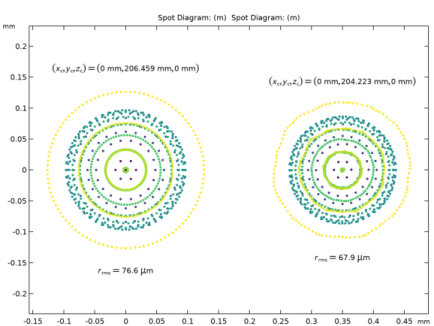
Click to expand the Focal Plane Orientation section. Click Create Focal Plane Dataset. This will create an Intersection Point 3D dataset on the plane that minimizes the RMS spot size.
|
|
5
|
|
6
|
|
7
|
|
1
|
|
2
|
|
3
|
|
4
|
|
5
|
|
1
|
In the Model Builder window, under Results>Spot Diagrams right-click Spot Diagram 1 and choose Duplicate.
|
|
2
|
|
3
|
|
4
|
Locate the Focal Plane Orientation section. Click Create Focal Plane Dataset. As before, this action will create another Intersection Point 3D dataset.
|
|
5
|
|
6
|