|
1
|
|
-
|
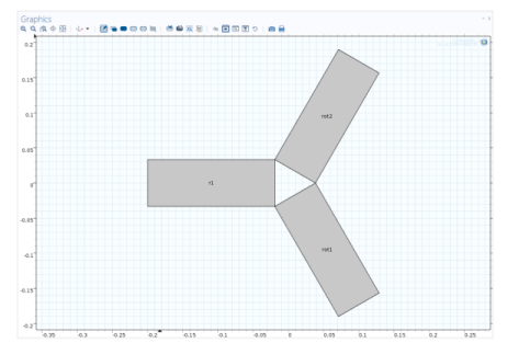
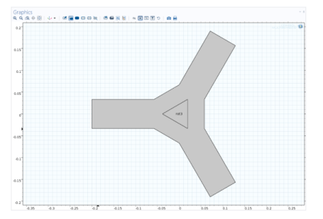
In the Width text field, enter 0.2-0.1/(3*sqrt(3)).
|
|
-
|
|
-
|
|
-
|
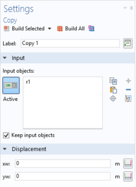
In the yw text field, enter -0.1/3.
|
|
3
|
|
2
|
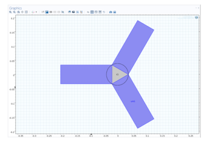
In the Settings window for Circle under Size and Shape, enter 0.2/(3*sqrt(3)) in the Radius text field.
|
|
1
|
|
2
|
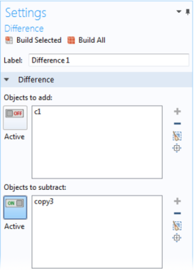
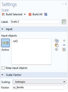
Go to the Settings window for Scale. Under Scale Factor in the Factor text field, enter sc_chamfer (one of the parameters entered in the step Global Definitions - Parameters and Variables).
|
|
3
|
|
2
|
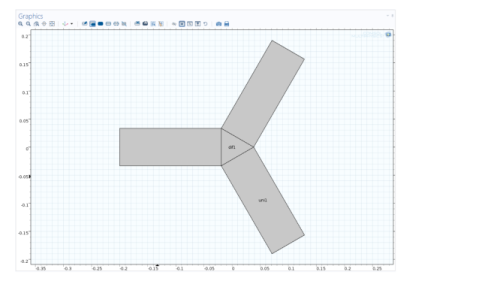
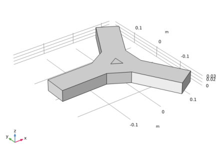
Go to the Settings window for Extrude. Under Distances from Plane in the associated table, enter 0.1/3 in the Distances (m) column.
|