Manufacturers usually provide curves that describe the static pressure as a function of flow rate for a fan. See Fan and Grille for the node settings.

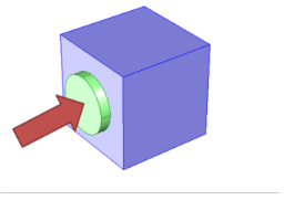
In this case, the device’s inlet is an external boundary, represented by the external circular boundary of the green domain on Figure 4-4. The device’s outlet is an interior face situated between the green and blue domains in Figure 4-4. The lumped curve gives the flow rate as a function of the pressure difference between the external boundary and the interior face. This boundary condition implementation follows the Pressure Boundary Condition for inlets with the Suppress backflow option:

Here, V0 is the flow rate across the boundary, pinput is the pressure at the device’s inlet, and Δpfan(V0) and Δpgrille(V0) are the static pressure functions of flow rate for the fan and the grille. Equation 4-48 and Equation 4-49 correspond to the compressible formulation. For incompressible flows, the term −(2/3)μ(∇ ⋅ u) vanishes. When a turbulence model with a transport equation for the turbulent kinetic energy is applied, the term −(2/3)ρk appears on the left-hand sides of Equation 4-48 and Equation 4-49. In such cases the turbulent kinetic energy, k, the turbulent relative fluctuations, ζ (for the v2-f turbulence model), and dissipation rate, ε, or specific dissipation rate, ω, must be specified on the downstream side. The turbulence conditions are specific to the design and operating conditions of the fan or grille. For the Fan condition, a reference velocity scale Uref is available in order to set default values according to Equation 4-47. For the Grille boundary condition the turbulence quantities on the downstream side are specified by defining a loss coefficient , from which a refraction coefficient is derived using Equation 4-62. Equation 4-55 through Equation 4-57 are then used to relate upstream and downstream turbulence quantities.

The flow direction is enforced to be normal to the boundary by default. However, it is possible to define an arbitrary inflow velocity direction. In such case, Equation 4-48 and Equation 4-49 are modified similarly to Equation 4-45. In 2D, the thickness in the third direction, Dz, is used to define the flow rate. Fans are modeled as rectangles in this case.

Here, the swirl ratio csf is a positive number less than 1, defining the ratio of the rotation transferred from the fan to the flow, f is the number of revolutions per time for the fan, and rbp is the rotation axis base point.

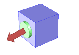
In this case (see Figure 4-14), the fan’s inlet is the interior face situated between the blue (cube) and green (circle) domain while its outlet is an external boundary, here the circular boundary of the green domain. The lumped curve gives the flow rate as a function of the pressure difference between the interior face and the external boundary. This boundary condition implementation follows the Pressure Boundary Condition for outlets with the Suppress backflow option:

Here, V0 is the flow rate across the boundary, pexit is the pressure at the device outlet, and Δpfan(V0) and Δpgrille(V0) are the static pressure function of flow rate for the fan and the grille. Equation 4-50 and Equation 4-51 correspond to the compressible formulation. For incompressible flows, the term −(2/3)μ(∇ ⋅ u)n vanishes. When a turbulence model with a transport equation for the turbulence kinetic energy is applied, the term −(2/3)ρkn appears on the left-hand sides of Equation 4-50 and Equation 4-51. In 2D the thickness in the third direction, Dz, is used to define the flow rate. Fans are modeled as rectangles in this case.