COMSOL 6.4 - Gaussian Beam Incident at the Brewster Angle

Gaussian Beam Incident at the Brewster Angle

For a plane wave incident at an interface between two different media, there exists an angle of incidence for which there is no reflectance if the incident wave is polarized in the plane of incidence. The angle, for which the reflectance is zero, is called the Brewster angle.

Figure 1 shows an incident wave being reflected and refracted at the interface between the two media. The polarization component polarized in the plane of incident (the plane spanned by the wave vector of the incident wave and the normal to the interface) is not reflected. This polarization component is called the p-polarization.

The polarization component orthogonal to the plane of incidence (the s-polarization) is both reflected and refracted.

Figure 1: The figure shows the incident, reflected, and refracted waves. At the Brewster angle αB the wave polarized in the plane of incidence is only refracted and not reflected.

At the Brewster angle, the incident p-polarized wave creates a polarization in the second medium (where the refracted wave is propagating) with the components in the propagation direction of the reflected wave. Because this is a longitudinal polarization for the reflected wave, and not a transverse polarization, it is clear that this polarization cannot excite a reflected wave.

Referring to the angles defined in Figure 1, write Snell’s law as

(1)

where n1 and n2 are the refractive indices above and below the interface, respectively.

Equation 1 results in the Brewster angle definition

From the Fresnel Equations Application Libraries example, the reflectance for the s-polarization at the Brewster angle is given by

(2)

This model does not use plane waves, but Gaussian beams (see for instance the Second Harmonic Generation of a Gaussian Beam Application Libraries model for a discussion about Gaussian beams). However, because the spot size for the beam is much larger than the wavelength, the plane wave relations above are good approximations also for the Gaussian beams.

Model Definition

This model demonstrates how the Matched Boundary Condition feature can be used to absorb waves that propagate toward a boundary in a direction different from the boundary’s normal direction. Here, a Scattering Boundary Condition feature is not an option, as that feature only absorbs waves propagating at or close to the normal direction to the boundary normal. A second alternative would be to use a Perfectly Matched Layer (PML) domain. However, in that case, extra degrees of freedom would have to be included for the PML domain. Thus, the Matched Boundary Condition feature is the best feature to use for absorbing beams propagating in directions that are not in the normal direction to the boundary.

Results and Discussion

First, the results are computed for s-polarization, where the polarization is orthogonal to the plane of incidence (out-of-plane polarization). As shown in Figure 2, there are both a refracted and a reflected beam. The incident beam and the reflected beam form an inference pattern. Thanks to the fine mesh used in the model, the interference pattern is resolved. Equation 2 is also used to verify that the reflectance is correct. It should be close to 14.8%.

Figure 2: The incident, transmitted (refracted) and reflected Gaussian beams for s-polarization (out-of-plane polarization).

Figure 3 shows the results for p-polarization (in-plane polarization). As expected, when the beam is incident at the Brewster angle, there is no reflected beam, but only a refracted (transmitted) beam.

Figure 3: The incident and transmitted Gaussian beams for p-polarization (in-plane polarization). For this polarization, with Brewster angle incidence, the reflected beam is gone.

Wave_Optics_Module/Beam_Propagation/brewster_interface

Modeling Instructions

From the menu, choose .

New

In the window, click

Model Wizard

In the window, click

In the tree, select > > .

Click .

Click

In the tree, select > .

Click

Global Definitions

Parameters 1

The parameters for the model will be read from a file.

In the window, under click .

In the window for , locate the section.

Click

Browse to the model’s Application Libraries folder and double-click the file brewster_interface.txt.

Geometry 1

Define the geometry as a rectangle with a diagonal boundary.

Rectangle 1 (r1)

In the toolbar, click

In the window for , locate the section.

In the text field, type b.

In the text field, type a.

Line Segment 1 (ls1)

In the toolbar, click

and choose .

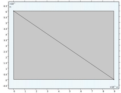
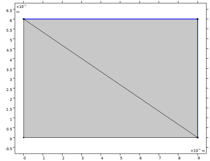
On the object , select Point 4 only.

In the window for , locate the section.

Click to select the

toggle button for .

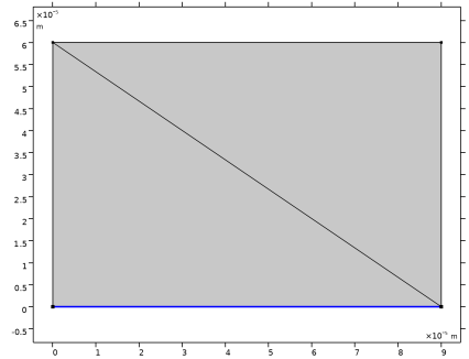
On the object , select Point 2 only.

Click

Click the

button in the toolbar.

Add Material

In the toolbar, click

to open the window.

The leftmost part consists of air and the rightmost part will be glass.

Go to the window.

In the tree, select > .

Click the button in the window toolbar.

In the toolbar, click

to close the window.

Materials

Glass

In the window, under right-click and choose .

In the window for , type Glass in the text field.

Select Domain 2 only.

Click the

button in the toolbar.

Define the refractive index for glass, using the parameter n2.

Locate the section. In the table, enter the following settings:


Property	Variable	Value	Unit	Property group
Refractive index, real part	n_iso ; nii = n_iso, nij = 0	n2	1	Refractive index

Definitions

Set up expressions for the wave vector components for the two waves, with different expressions in the two domains.

Variables 1

In the window, under right-click and choose .

In the window for , locate the section.

From the list, choose .

Select Domain 1 only.

Locate the section. In the table, enter the following settings:


Name	Expression	Unit	Description
k1x	k1x_air	1/m	Wave vector, first wave, x-component
k1y	k1y_air	1/m	Wave vector, first wave, y-component
k2x	k2x_air	1/m	Wave vector, second wave, x-component
k2y	k2y_air	1/m	Wave vector, second wave, y-component

Variables 2

In the toolbar, click

In the window for , locate the section.

From the list, choose .

Select Domain 2 only.

Locate the section. In the table, enter the following settings:


Name	Expression	Unit	Description
k1x	k1x_glass	1/m	Wave vector, first wave, x-component
k1y	k1y_glass	1/m	Wave vector, first wave, y-component
k2x	k2x_glass	1/m	Wave vector, second wave, x-component
k2y	k2y_glass	1/m	Wave vector, second wave, y-component

Electromagnetic Waves, Beam Envelopes (ewbe)

In the window, under click .

In the window for , locate the section.

From the list, choose .

Locate the section. Specify the k1 vector as


k1x	x
k1y	y

Specify the k2 vector as


k2x	x
k2y	y

Matched Boundary Condition 1

In the toolbar, click

and choose .

Select Boundary 1 only.

In the window for , locate the section.

From the list, choose .

In the w0 text field, type w0.

Specify the Eg0 vector as


0	x
0	y
1[V/m]	z

On this boundary, only an incident field is expected, but there should not be any scattered field. Thus, provide that information, with the following setting, to avoid any potential spurious solutions.

Find the subsection. Select the checkbox.

On the rightmost boundary, a transmitted Gaussian beam, propagating at an angle to the boundary normal, is expected. Thus, add a Matched Boundary Condition feature that will absorb this transmitted Gaussian beam.

Matched Boundary Condition 2

In the toolbar, click

and choose .

Select Boundaries 4 and 5 only.

In the window for , locate the section.

From the list, choose .

The reflected wave, propagating toward the bottom boundary, will also propagate at an angle to the normal to the bottom boundary. Thus, add a Matched Boundary Condition feature here, too, to absorb the reflected beam.

Matched Boundary Condition 3

In the toolbar, click

and choose .

Select Boundary 2 only.

Definitions

Set up integration operators to calculate the power of the incident, reflected, and transmitted beams.

Integration 1 (intop1)

In the toolbar, click

and choose .

In the window for , locate the section.

From the list, choose .

Select Boundary 1 only.

Integration 2 (intop2)

In the toolbar, click

and choose .

In the window for , locate the section.

From the list, choose .

Select Boundaries 4 and 5 only.

Integration 3 (intop3)

In the toolbar, click

and choose .

In the window for , locate the section.

From the list, choose .

Select Boundary 2 only.

Variables 3

Now, define the power variables for the beams, using the previously defined integration operators.

In the window, right-click and choose .

In the window for , locate the section.

In the table, enter the following settings:


Name	Expression	Unit	Description
Pin	-intop1(ewbe.nPoav)	W/m	Input power
Pt	intop2(ewbe.nPoav)	W/m	Transmitted power
Pr	intop3(ewbe.nPoav)	W/m	Reflected power

The minus sign for the input power is used as the power flow and the boundary normal point in the opposite directions.

Mesh 1

Let the physics define a triangular mesh where the maximum mesh element size is set to half a wavelength, to resolve the interference pattern created by the incident and the reflected beam.

In the window, under click .

In the window for , locate the section.

From the list, choose .

In the hmax text field, type lda0/2.

Study 1

Step 1: Frequency Domain

Define the frequency and compute the solution for the model.

In the window, under click .

In the window for , locate the section.

In the text field, type f0.

In the toolbar, click

Results

Electric Field, First Wave (ewbe)

This is the electric field norm of the first wave for s-polarization.

Electric Field, Second Wave (ewbe)

In the window, click .

This is the electric field norm of the second wave for s-polarization.

Electric Field (ewbe)

Right-click and choose .

In the window for , type Electric Field (ewbe) in the text field.

Electric Field

In the window, expand the node, then click .

In the window for , locate the section.

In the text field, type ewbe.normE.

To really resolve the inference pattern to the left of the air-glass interface, set the resolution to extra fine.

Click to expand the section. From the list, choose .

From the list, choose .

In the toolbar, click

Click the

button in the toolbar. Compare your result with the plot below.

Using the defined variables, compute the reflectance.

Global Evaluation 1

In the toolbar, click

In the window for , locate the section.

In the table, enter the following settings:


Expression	Unit	Description
Pr/Pin	1

Click

Table 1

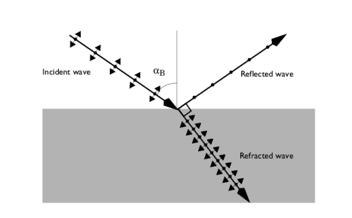
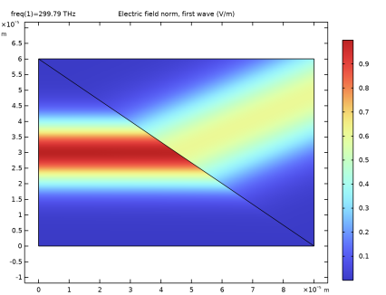
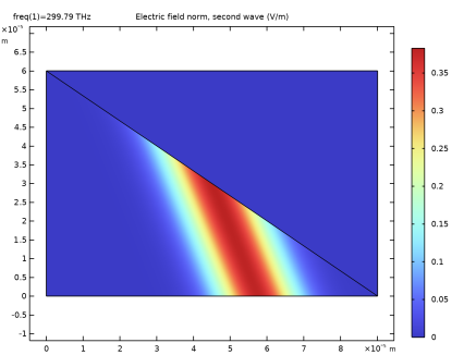
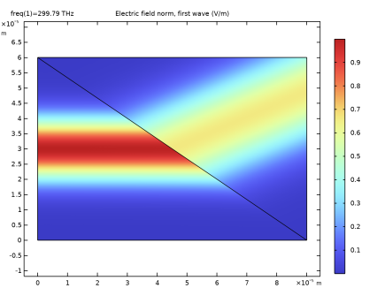
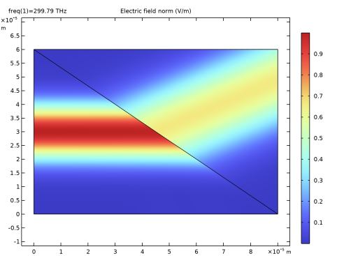
Go to the window. Compare the calculated reflectance with the theoretical value for s-polarized plane waves. Notice that the values are almost the same.

In the window for , locate the section.

In the table, enter the following settings: