
|
|
|


|
|
|||


|
1
|
|
2
|
|
3
|
Click Add.
|
|
4
|
Click
|
|
5
|
|
6
|
Click
|
|
1
|
|
2
|
|
3
|
Click
|
|
4
|
Browse to the model’s Application Libraries folder and double-click the file microwave_cavity_plasma_parameters.txt.
|
|
1
|
In the Model Builder window, under Component 1 (comp1) right-click Definitions and choose Variables.
|
|
2
|
|
1
|
|
2
|
|
3
|
|
1
|
|
2
|
|
3
|
|
4
|
|
1
|
|
2
|
|
3
|
|
4
|
|
1
|
|
2
|
|
3
|
|
4
|
|
5
|
|
1
|
|
2
|
|
3
|
|
4
|
|
5
|
|
1
|
|
2
|
|
3
|
|
4
|
|
5
|
|
1
|
|
2
|
|
3
|
|
4
|
|
1
|
|
2
|
|
3
|
|
4
|
|
5
|
|
6
|
|
7
|
|
1
|
|
2
|
|
3
|
|
4
|
|
5
|
|
6
|
|
7
|
Click
|
|
1
|
|
2
|
|
3
|
|
4
|
|
1
|
|
2
|
|
3
|
|
4
|
|
5
|
|
1
|
|
2
|
|
1
|
|
2
|
|
3
|
|
4
|
Clear the Keep interior boundaries checkbox.
|
|
5
|
Click
|
|
1
|
|
2
|
|
3
|
|
4
|
|
5
|
|
6
|
|
7
|
|
1
|
|
2
|
|
3
|
On the object r7, select Points 1–4 only.
|
|
4
|
|
5
|
|
1
|
|
2
|
|
3
|
|
4
|
|
5
|
|
1
|
|
2
|
Select the object uni1 only.
|
|
3
|
|
4
|
|
5
|
|
1
|
|
2
|
|
3
|
|
4
|
|
1
|
|
2
|
|
3
|
|
4
|
On the object ca3, select Point 1 only.
|
|
5
|
|
6
|
On the object r4, select Point 2 only.
|
|
1
|
|
2
|
On the object ls2, select Point 1 only.
|
|
3
|
|
4
|
|
5
|
On the object thi1(3), select Point 2 only.
|
|
1
|
|
2
|
On the object dif1, select Point 9 only.
|
|
3
|
|
4
|
|
1
|
|
2
|
|
3
|
|
4
|
|
5
|
|
1
|
|
2
|
On the object fin, select Boundaries 4, 22, 23, 26, and 38 only.
|
|
3
|
|
4
|
|
a
|
Species properties using Preset species data
|
|
1
|
|
2
|
|
3
|
Click
|
|
4
|
Browse to the model’s Application Libraries folder and double-click the file H2_plasma_chemistry.txt.
|
|
5
|
Click
|
|
1
|
|
2
|
Go to the Add Material window.
|
|
3
|
|
4
|
Click the Add to Component button in the window toolbar.
|
|
5
|
|
6
|
Click the Add to Component button in the window toolbar.
|
|
7
|
|
1
|
|
2
|
|
3
|
Select the Full expression for diffusivity checkbox.
|
|
4
|
Select the Mixture diffusion correction checkbox.
|
|
5
|
Locate the Plasma Properties section. Select the Use reduced electron transport properties checkbox.
|
|
6
|
Locate the Electron Energy Distribution Function Settings section. From the Electron energy distribution function list, choose Generalized.
|
|
7
|
|
8
|
|
1
|
In the Model Builder window, expand the Component 1 (comp1) > Plasma (plas) > Group - Species node, then click Species: H2.
|
|
2
|
|
3
|
Select the From mass constraint checkbox.
|
|
1
|
|
2
|
|
3
|
|
1
|
|
2
|
|
3
|
|
1
|
|
2
|
|
3
|
|
1
|
|
2
|
|
3
|
|
1
|
|
2
|
|
3
|
Select the Initial value from electroneutrality constraint checkbox.
|
|
1
|
|
3
|
|
4
|
|
5
|
|
1
|
|
2
|
|
3
|
|
1
|
In the Model Builder window, expand the Component 1 (comp1) > Plasma (plas) > Group - Surface Reactions node, then click 1: H=>0.5H2.
|
|
2
|
|
3
|
|
1
|
|
2
|
|
3
|
|
1
|
|
2
|
|
3
|
|
1
|
|
2
|
|
3
|
|
1
|
|
2
|
|
3
|
|
1
|
|
2
|
|
3
|
|
1
|
|
1
|
|
2
|
|
3
|
|
1
|
|
1
|
|
2
|
|
3
|
Click
|
|
5
|
|
1
|
|
3
|
|
4
|
From the list, choose Mass flow.
|
|
5
|
|
6
|
|
1
|
|
1
|
|
2
|
|
3
|
Click
|
|
1
|
In the Model Builder window, under Component 1 (comp1) > Heat Transfer in Fluids (ht) click Initial Values 1.
|
|
2
|
|
3
|
|
1
|
|
3
|
|
4
|
|
1
|
|
3
|
|
4
|
|
1
|
|
2
|
|
3
|
|
4
|
|
5
|
|
1
|
|
1
|
|
3
|
|
4
|
|
5
|
|
1
|
|
2
|
|
3
|
|
1
|
|
1
|
|
2
|
|
3
|
|
4
|
|
1
|
|
2
|
|
3
|
|
1
|
|
2
|
|
3
|
|
4
|
|
1
|
|
2
|
|
3
|
|
5
|
|
6
|
|
7
|
Click the Custom button.
|
|
8
|
Locate the Element Size Parameters section.
|
|
9
|
|
1
|
|
2
|
|
3
|
|
5
|
|
6
|
|
7
|
Click the Custom button.
|
|
8
|
Locate the Element Size Parameters section.
|
|
9
|
|
1
|
|
2
|
|
3
|
|
5
|
|
6
|
|
7
|
Click the Custom button.
|
|
8
|
Locate the Element Size Parameters section.
|
|
9
|
|
1
|
|
2
|
|
3
|
Click the Custom button.
|
|
4
|
Locate the Element Size Parameters section.
|
|
5
|
|
6
|
|
1
|
|
2
|
|
3
|
Clear the Smooth transition to interior mesh checkbox.
|
|
4
|
Click to expand the Corner Settings section. Locate the Domain Selection section. From the Geometric entity level list, choose Domain.
|
|
1
|
|
2
|
|
3
|
|
5
|
|
1
|
|
2
|
|
3
|
In the Solve for column of the table, under Component 1 (comp1), clear the checkbox for Laminar Flow (spf).
|
|
4
|
|
5
|
|
6
|
|
7
|
|
8
|
|
9
|
Click Replace.
|
|
10
|
|
11
|
|
12
|
|
13
|
|
1
|
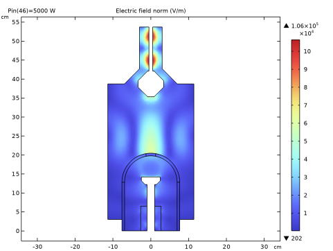
In the Model Builder window, under Results, Ctrl-click to select Electron Density (plas), Electron Temperature (plas), Electric Potential (plas), Temperature (ht), and Electric Field (emw).
|
|
2
|
Right-click and choose Group.
|
|
1
|
|
2
|
|
1
|
|
2
|
|
3
|
Select the Plot checkbox.
|
|
4
|
|
5
|
|
1
|
|
2
|
Go to the Add Study window.
|
|
3
|
Find the Studies subsection. In the Select Study tree, select Preset Studies for Selected Multiphysics > Frequency–Stationary.
|
|
4
|
Click the Add Study button in the window toolbar.
|
|
5
|
|
1
|
|
2
|
|
3
|
Click to expand the Values of Dependent Variables section. Find the Initial values of variables solved for subsection. From the Settings list, choose User controlled.
|
|
4
|
|
5
|
|
6
|
|
7
|
Click
|
|
8
|
Click
|
|
9
|
|
10
|
|
11
|
|
12
|
Click Replace.
|
|
13
|
|
14
|
|
15
|
|
16
|
|
1
|
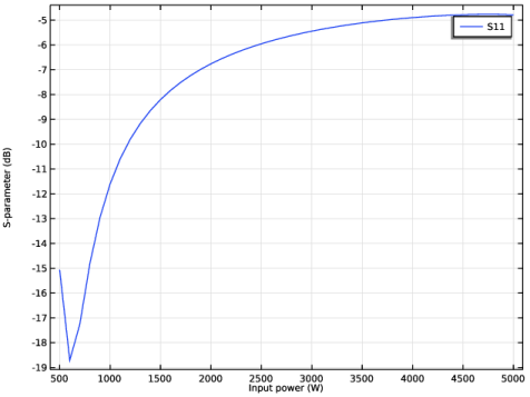
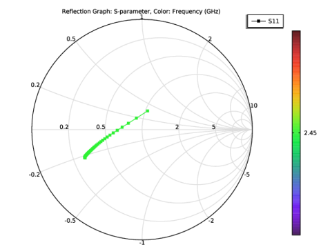
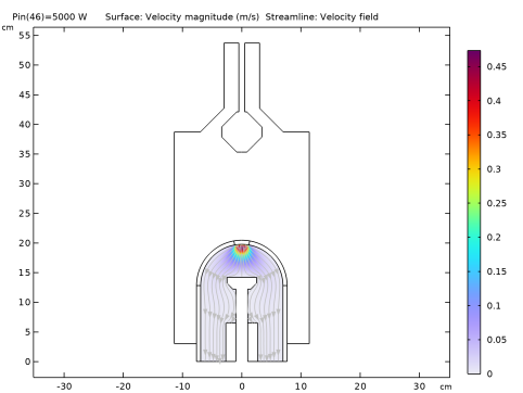
In the Model Builder window, under Results, Ctrl-click to select Electron Density (plas) 1, Electron Temperature (plas) 1, Electric Potential (plas) 1, Velocity (spf), Pressure (spf), Velocity, 3D (spf), Temperature (ht) 1, Electric Field (emw) 1, S-Parameter (emw), and Smith Plot (emw).
|
|
2
|
Right-click and choose Group.
|
|
1
|
|
2
|
|
1
|
|
2
|
|
3
|
Select the Plot checkbox.
|
|
5
|
|
1
|
|
2
|
|
3
|
|
4
|
|
5
|
Click to expand the Advanced section. Find the Space variables subsection. Select the Remove elements on the symmetry axis checkbox.
|
|
1
|
|
2
|
|
3
|
|
4
|
|
1
|
|
2
|
|
3
|
|
4
|
|
1
|
|
2
|
|
3
|
|
4
|
|
1
|
|
2
|
|
3
|
|
4
|
|
1
|
|
2
|
|
3
|
|
1
|
|
2
|
|
3
|
|
4
|
|
5
|
|
6
|
Locate the Coloring and Style section. Find the Point style subsection. From the Type list, choose Arrow.
|
|
7
|
|
8
|
|
9
|
|
1
|
|
2
|
|
3
|
|
4
|
|
1
|
|
2
|
|
3
|
|
4
|
|
1
|
|
2
|
|
3
|
|
4
|
|
5
|
|
1
|
|
2
|
|
3
|
|
4
|
|
1
|
|
2
|
|
3
|
|
4
|
|
1
|
|
2
|
|
3
|
|
4
|
|
1
|
|
2
|
|
3
|
|
4
|
|
1
|
|
3
|