
|
|
|


|
|
|||
|
1
|
|
2
|
|
3
|
Click Add.
|
|
4
|
Click
|
|
5
|
|
6
|
Click
|
|
1
|
|
2
|
|
3
|
|
1
|
|
2
|
|
1
|
In the Model Builder window, under Component 1 (comp1) right-click Definitions and choose Variables.
|
|
2
|
|
1
|
|
2
|
|
3
|
|
5
|
|
6
|
|
7
|
In the Argument table, enter the following settings:
|
|
1
|
|
2
|
|
3
|
|
4
|
|
5
|
Click
|
|
1
|
|
2
|
|
3
|
|
4
|
Click to expand the Heavy Species Energy Balance section. Select the Include heavy species energy conservation equation checkbox.
|
|
5
|
|
1
|
|
2
|
|
3
|
|
4
|
|
5
|
|
6
|
|
7
|
|
1
|
|
2
|
|
3
|
Click
|
|
4
|
Browse to the model’s Application Libraries folder and double-click the file H2_plasma_chemistry.txt.
|
|
5
|
Click
|
|
1
|
In the Model Builder window, expand the Component 1 (comp1) > Plasma (plas) > Group - Species node, then click Species: H2.
|
|
2
|
|
3
|
Select the From mass constraint checkbox.
|
|
4
|
|
1
|
In the Model Builder window, expand the Component 1 (comp1) > Plasma (plas) > Group - Surface Reactions node, then click 1: H=>0.5H2.
|
|
3
|
|
4
|
|
5
|
|
1
|
|
2
|
|
3
|
|
4
|
Locate the Reaction Formula section. From the Specify reaction using list, choose Sticking coefficient and diffusion.
|
|
5
|
|
1
|
|
2
|
|
3
|
|
4
|
Locate the Reaction Formula section. From the Specify reaction using list, choose Sticking coefficient and diffusion.
|
|
5
|
|
1
|
|
2
|
|
3
|
|
4
|
|
5
|
|
1
|
|
2
|
|
3
|
|
4
|
|
5
|
|
1
|
|
2
|
|
3
|
|
4
|
|
5
|
|
1
|
|
2
|
|
3
|
|
1
|
|
2
|
|
3
|
Clear the Generate default plots checkbox.
|
|
1
|
|
2
|
|
3
|
Select the Auxiliary sweep checkbox.
|
|
4
|
Click
|
|
6
|
|
7
|
|
8
|
|
1
|
|
2
|
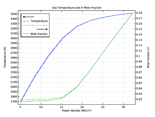
In the Settings window for 1D Plot Group, type Gas Temperature and H Mole Fraction in the Label text field.
|
|
1
|
|
2
|
|
4
|
|
5
|
|
6
|
|
1
|
|
2
|
|
1
|
|
2
|
|
3
|
|
4
|
Locate the Plot Settings section.
|
|
5
|
Select the x-axis label checkbox. In the associated text field, type Power density (W/cm<sup>3</sup>).
|
|
6
|
Select the Two y-axes checkbox.
|
|
7
|
|
8
|
|
1
|
|
2
|
|
1
|
|
2
|
|
4
|
|
5
|
|
6
|
|
7
|
|
8
|
Select the Expression checkbox.
|
|
9
|
|
1
|
|
2
|
|
3
|
|
4
|
Locate the Plot Settings section.
|
|
5
|
Select the x-axis label checkbox. In the associated text field, type Power density (W/cm<sup>3</sup>).
|
|
6
|
|
7
|
Select the Manual axis limits checkbox.
|
|
8
|
|
9
|
|
10
|
|
1
|
|
2
|
|
1
|
|
2
|
|
4
|
|
5
|
|
6
|
|
7
|
|
1
|
|
2
|
|
3
|
|
4
|
Locate the Plot Settings section.
|
|
5
|
Select the x-axis label checkbox. In the associated text field, type Power density (W/cm<sup>3</sup>).
|
|
6
|
|
7
|
|
8
|
|
9
|
|
10
|
|
1
|
|
2
|
|
1
|
|
2
|
|
4
|
|
5
|
|
6
|
|
7
|
|
8
|
Select the Expression checkbox.
|
|
9
|
|
1
|
|
2
|
|
3
|
|
4
|
Locate the Plot Settings section.
|
|
5
|
Select the x-axis label checkbox. In the associated text field, type Power density (W/cm<sup>3</sup>).
|
|
6
|
|
7
|
|
1
|
|
2
|
|
1
|
|
2
|
|
4
|
|
5
|
|
6
|
|
7
|
|
8
|
|
1
|
|
2
|
|
3
|
|
4
|
Locate the Plot Settings section.
|
|
5
|
Select the x-axis label checkbox. In the associated text field, type Power density (W/cm<sup>3</sup>).
|
|
6
|
|
7
|
|
8
|
Select the Manual axis limits checkbox.
|
|
9
|
|
10
|
|
11
|
|
1
|
|
2
|
|
3
|
In the Settings window for Plasma, locate the Electron Energy Distribution Function Settings section.
|
|
4
|
From the Electron energy distribution function list, choose Boltzmann equation, two-term approximation (linear).
|
|
5
|
Select the Oscillating field checkbox.
|
|
6
|
|
7
|
|
1
|
|
2
|
Go to the Add Study window.
|
|
3
|
Find the Studies subsection. In the Select Study tree, select Preset Studies for Selected Physics Interfaces > EEDF Initialization.
|
|
4
|
Click the Add Study button in the window toolbar.
|
|
5
|
|
6
|
Click the Add Study button in the window toolbar.
|
|
7
|
|
1
|
|
2
|
|
3
|
Find the Initial values of variables solved for subsection. From the Settings list, choose User controlled.
|
|
4
|
|
5
|
|
6
|
|
7
|
Click
|
|
9
|
|
10
|
|
11
|
|
12
|
|
13
|
Clear the Generate default plots checkbox.
|
|
14
|
|
15
|
|
16
|
|
1
|
|
2
|
|
1
|
|
2
|
|
3
|
|
1
|
In the Model Builder window, under Results > Gas Temperature and H Mole Fraction right-click Global 1 and choose Duplicate.
|
|
2
|
|
3
|
|
4
|
Click to expand the Coloring and Style section. Find the Line style subsection. From the Line list, choose Dashed.
|
|
5
|
|
6
|
|
1
|
In the Model Builder window, under Results > Gas Temperature and H Mole Fraction right-click Global 2 and choose Duplicate.
|
|
2
|
|
3
|
|
4
|
Locate the Coloring and Style section. Find the Line style subsection. From the Line list, choose Dashed.
|
|
5
|
|
1
|
In the Model Builder window, under Results > Ions Density right-click Global 1 and choose Duplicate.
|
|
2
|
|
3
|
|
4
|
Locate the Coloring and Style section. Find the Line style subsection. From the Line list, choose Dashed.
|
|
5
|
|
6
|
|
7
|
|
1
|
In the Model Builder window, under Results > Electron Temperature right-click Global 1 and choose Duplicate.
|
|
2
|
|
3
|
|
4
|
Locate the y-Axis Data section. In the table, enter the following settings:
|
|
5
|
|
1
|
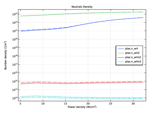
In the Model Builder window, under Results > Neutrals Density right-click Global 1 and choose Duplicate.
|
|
2
|
|
3
|
|
4
|
Locate the Coloring and Style section. Find the Line style subsection. From the Line list, choose Dashed.
|
|
5
|
|
6
|
|
1
|
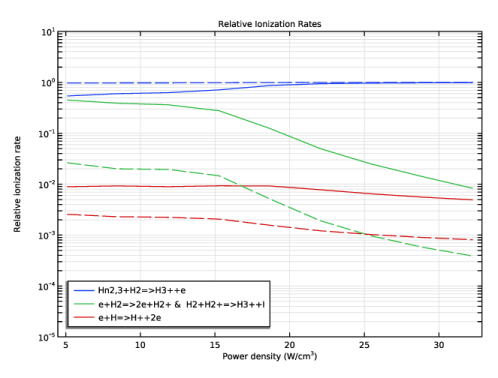
In the Model Builder window, under Results > Relative Ionization Rates right-click Global 1 and choose Duplicate.
|
|
2
|
|
3
|
|
4
|
Locate the Coloring and Style section. Find the Line style subsection. From the Line list, choose Dashed.
|
|
5
|
|
6
|
|
1
|
|
2
|
|
3
|
|
4
|
|
1
|
|
2
|
|
3
|
|
4
|
|
1
|
|
2
|
|
3
|
|
4
|
|
5
|
|
6
|
|
7
|
|
8
|
|
9
|
|
10
|
|
1
|
|
2
|
|
3
|
|
4
|
|
5
|
|
6
|
|
7
|
|
1
|
|
2
|
|
3
|
|
4
|
Locate the Plot Settings section.
|
|
5
|
|
6
|
|
7
|
|
8
|
Select the Manual axis limits checkbox.
|
|
9
|
|
10
|
|
11
|
|
12
|
|
13
|
 .
.