|
|
|


|
1
|
|
2
|
|
3
|
Click Add.
|
|
4
|
Click
|
|
5
|
|
6
|
Click
|
|
1
|
|
2
|
Browse to the model’s Application Libraries folder and double-click the file small_concert_hall_geom_sequence.mph.
|
|
3
|
|
4
|
|
5
|
|
6
|
|
1
|
|
2
|
|
3
|
|
4
|
Browse to the model’s Application Libraries folder and double-click the file small_concert_hall_parameters_model.txt.
|
|
1
|
|
2
|
In the Settings window for Parameters, type Parameters 2 - Source and Receiver Positions in the Label text field.
|
|
3
|
|
4
|
Browse to the model’s Application Libraries folder and double-click the file small_concert_hall_parameters_source_positions.txt.
|
|
1
|
|
2
|
In the Settings window for Parameters, type Parameters 3 - Source and Receiver Settings in the Label text field.
|
|
3
|
|
4
|
Browse to the model’s Application Libraries folder and double-click the file small_concert_hall_parameters_source_settings.txt.
|
|
1
|
|
2
|
|
3
|
|
4
|
Click
|
|
5
|
Browse to the model’s Application Libraries folder and double-click the file small_concert_hall_radiation_balloon.txt.
|
|
6
|
Click
|
|
7
|
Locate the Data Column Settings section. In the table, click to select the cell at row number 1 and column number 1.
|
|
8
|
|
10
|
|
12
|
|
14
|
|
15
|
|
17
|
|
18
|
|
1
|
|
2
|
|
3
|
|
4
|
Click
|
|
5
|
Browse to the model’s Application Libraries folder and double-click the file small_concert_hall_absorption_parameters.txt.
|
|
6
|
Click
|
|
7
|
Locate the Data Column Settings section. In the table, enter the following settings:
|
|
9
|
|
11
|
|
12
|
|
14
|
|
15
|
|
17
|
|
18
|
|
20
|
|
21
|
|
23
|
|
24
|
|
26
|
|
27
|
|
29
|
|
30
|
|
1
|
|
2
|
|
3
|
|
4
|
Click
|
|
5
|
Browse to the model’s Application Libraries folder and double-click the file small_concert_hall_air_attenuation.txt.
|
|
6
|
Click
|
|
7
|
|
8
|
Locate the Interpolation and Extrapolation section. From the Interpolation list, choose Nearest neighbor.
|
|
9
|
|
10
|
In the Function table, enter the following settings:
|
|
1
|
|
2
|
|
3
|
|
4
|
|
5
|
|
1
|
|
2
|
|
3
|
|
4
|
|
5
|
|
1
|
|
2
|
|
3
|
|
4
|
|
5
|
|
6
|
|
7
|
|
8
|
Locate the Selections of Resulting Entities section. Select the Resulting objects selection checkbox.
|
|
9
|
|
10
|
|
1
|
|
2
|
|
3
|
|
4
|
|
5
|
|
1
|
|
2
|
|
3
|
|
4
|
|
1
|
|
2
|
|
3
|
|
4
|
|
1
|
|
2
|
|
3
|
|
4
|
|
1
|
|
2
|
|
3
|
|
4
|
|
1
|
|
2
|
|
3
|
|
4
|
|
1
|
|
2
|
|
3
|
|
4
|
|
1
|
|
2
|
In the Settings window for Variables, type Variables: Quality Metric Estimates in the Label text field.
|
|
3
|
|
4
|
Browse to the model’s Application Libraries folder and double-click the file small_concert_hall_variables.txt.
|
|
1
|
|
2
|
|
3
|
|
4
|
Locate the Material Properties of Exterior and Unmeshed Domains section. In the cext text field, type c0.
|
|
5
|
|
6
|
|
1
|
In the Model Builder window, under Component 1 (comp1) > Ray Acoustics (rac) click Ray Properties 1.
|
|
2
|
|
3
|
|
1
|
|
2
|
|
3
|
|
4
|
|
5
|
|
1
|
|
2
|
|
3
|
|
4
|
|
5
|
|
1
|
|
2
|
|
3
|
|
4
|
|
5
|
|
1
|
|
2
|
|
3
|
|
4
|
|
5
|
|
1
|
|
2
|
|
3
|
|
4
|
|
5
|
|
1
|
|
2
|
|
3
|
|
4
|
|
5
|
|
1
|
|
2
|
|
3
|
|
5
|
|
6
|
|
1
|
|
2
|
|
3
|
Select the Compute smoothed accumulated variable checkbox.
|
|
1
|
|
2
|
|
3
|
|
5
|
|
6
|
|
1
|
|
2
|
|
3
|
|
4
|
|
5
|
|
6
|
|
7
|
|
1
|
|
2
|
|
3
|
|
4
|
|
5
|
|
6
|
Locate the Intensity and Power section. In the D(φθ,) text field, type 20*log10(abs(preal(rac.swd2.phi,rac.swd2.theta,f0)+i*pimag(rac.swd2.phi,rac.swd2.theta,f0))/sqrt(2)/20e-6[Pa]).
|
|
7
|
|
8
|
|
1
|
|
2
|
|
3
|
|
4
|
|
5
|
|
1
|
|
2
|
|
3
|
|
1
|
|
2
|
|
3
|
|
4
|
|
1
|
|
2
|
|
3
|
|
4
|
Clear the Minimum element size checkbox.
|
|
1
|
|
2
|
|
3
|
|
1
|
|
2
|
|
3
|
Click
|
|
5
|
|
6
|
Locate the Element Size Parameters section.
|
|
7
|
|
1
|
|
2
|
|
3
|
Click
|
|
4
|
|
5
|
Click OK.
|
|
6
|
|
1
|
|
2
|
|
1
|
|
2
|
|
3
|
|
4
|
|
5
|
Locate the Physics and Variables Selection section. Select the Modify model configuration for study step checkbox.
|
|
6
|
|
7
|
Click
|
|
1
|
|
2
|
|
3
|
Click
|
|
6
|
Click
|
|
7
|
|
8
|
|
9
|
|
10
|
Click Replace.
|
|
11
|
|
1
|
|
2
|
|
3
|
|
4
|
|
1
|
|
2
|
|
3
|
|
4
|
|
1
|
|
2
|
|
3
|
|
4
|
|
1
|
|
2
|
|
3
|
|
4
|
|
1
|
|
2
|
|
3
|
|
4
|
Click
|
|
5
|
|
6
|
|
7
|
|
8
|
Click Replace.
|
|
9
|
|
10
|
|
11
|
|
12
|
|
13
|
|
14
|
Select the Only plot when requested checkbox.
|
|
15
|
Select the Recompute all plot data after solving checkbox.
|
|
16
|
|
17
|
|
18
|
|
19
|
|
20
|
Click OK.
|
|
1
|
|
2
|
|
1
|
|
2
|
|
3
|
|
4
|
|
1
|
|
2
|
|
3
|
|
4
|
|
1
|
|
2
|
|
3
|
|
1
|
|
2
|
|
3
|
|
4
|
|
5
|
|
1
|
|
2
|
|
3
|
|
4
|
|
5
|
|
1
|
|
2
|
|
3
|
|
4
|
|
5
|
|
6
|
|
7
|
|
8
|
|
9
|
|
10
|
|
11
|
|
1
|
|
2
|
|
3
|
|
4
|
Click
|
|
5
|
Browse to the model’s Application Libraries folder and double-click the file small_concert_hall_impulse_response.wav.
|
|
6
|
Find the Functions subsection. In the table, enter the following settings:
|
|
7
|
|
8
|
In the Argument table, enter the following settings:
|
|
1
|
|
2
|
Expand the Impulse Response 1 node.
|
|
1
|
|
2
|
|
1
|
|
2
|
|
3
|
|
4
|
|
1
|
|
2
|
|
3
|
|
4
|
|
5
|
|
6
|
|
7
|
|
8
|
|
9
|
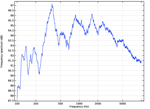
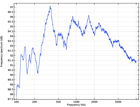
Select the Frequency range checkbox.
|
|
10
|
|
11
|
|
12
|
Select the In dB checkbox.
|
|
13
|
|
14
|
|
15
|
|
16
|
|
17
|
|
18
|
|
19
|
|
20
|
|
21
|
|
1
|
|
2
|
|
3
|
Locate the Data section. From the Dataset list, choose Study 1 - Omnidirectional Source/Parametric Solutions 1 (sol2).
|
|
4
|
|
1
|
|
2
|
In the Settings window for Surface, click Replace Expression in the upper-right corner of the Expression section. From the menu, choose Component 1 (comp1) > Ray Acoustics > Accumulated variables > Wall intensity comp1.rac.wall8.spl1.Iw > rac.wall8.spl1.Lp - Sound pressure level - dB.
|
|
3
|
|
4
|
|
1
|
|
2
|
|
3
|
|
4
|
Locate the Plot Settings section.
|
|
5
|
|
6
|
|
7
|
|
8
|
|
1
|
|
2
|
|
3
|
|
4
|
|
5
|
Click to expand the Coloring and Style section. Find the Line style subsection. From the Line list, choose None.
|
|
6
|
|
7
|
|
8
|
Select the Show legends checkbox.
|
|
1
|
|
2
|
|
3
|
|
4
|
Locate the Legends section. In the table, enter the following settings:
|
|
5
|
|
1
|
|
2
|
|
3
|
Locate the Data section. From the Dataset list, choose Study 1 - Omnidirectional Source/Parametric Solutions 1 (sol2).
|
|
4
|
|
5
|
|
6
|
Locate the Plot Settings section.
|
|
7
|
|
8
|
|
9
|
|
10
|
|
11
|
|
12
|
|
13
|
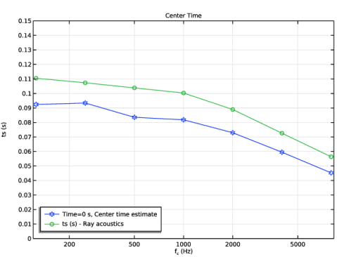
Select the x-axis log scale checkbox.
|
|
14
|
|
1
|
|
2
|
|
4
|
|
5
|
Click to expand the Coloring and Style section. Find the Line markers subsection. From the Marker list, choose Star.
|
|
1
|
|
2
|
|
3
|
|
4
|
|
5
|
|
6
|
Locate the Coloring and Style section. Find the Line markers subsection. From the Marker list, choose Circle.
|
|
7
|
|
8
|
|
9
|
|
1
|
|
2
|
|
3
|
Locate the Data section. From the Dataset list, choose Study 1 - Omnidirectional Source/Parametric Solutions 1 (sol2).
|
|
4
|
|
5
|
|
6
|
Locate the Plot Settings section.
|
|
7
|
|
8
|
|
9
|
|
10
|
|
11
|
|
12
|
|
13
|
|
14
|
Select the x-axis log scale checkbox.
|
|
15
|
|
1
|
|
2
|
|
4
|
|
5
|
Click to expand the Coloring and Style section. Find the Line markers subsection. From the Marker list, choose Star.
|
|
1
|
|
2
|
|
3
|
|
4
|
|
5
|
|
6
|
Locate the Coloring and Style section. Find the Line markers subsection. From the Marker list, choose Circle.
|
|
7
|
|
8
|
|
9
|
|
1
|
|
2
|
|
3
|
|
4
|
|
5
|
|
6
|
|
7
|
|
1
|
|
2
|
|
1
|
|
2
|
|
3
|
|
4
|
|
1
|
|
2
|
|
3
|
|
4
|
|
5
|
|
6
|
|
7
|
|
8
|
|
1
|
|
2
|
|
1
|
|
2
|
|
3
|
|
4
|
|
1
|
|
2
|
|
3
|
|
4
|
|
5
|
|
6
|
|
7
|
|
1
|
|
2
|
|
1
|
|
2
|
|
3
|
|
1
|
|
2
|
|
3
|
|
4
|
|
5
|
|
6
|
|
7
|
|
8
|
|
1
|
|
2
|
|
3
|
|
4
|
|
1
|
In the Model Builder window, under Results, Ctrl-click to select Definition, Clarity, Center Time, Reverberation Times, and Speech Transmission Index.
|
|
2
|
Right-click and choose Group.
|
|
1
|
|
2
|
Go to the Add Study window.
|
|
3
|
Find the Studies subsection. In the Select Study tree, select Preset Studies for Selected Physics Interfaces > Ray Tracing.
|
|
4
|
Click the Add Study button in the window toolbar.
|
|
5
|
|
1
|
|
2
|
|
3
|
|
4
|
|
5
|
Locate the Physics and Variables Selection section. Select the Modify model configuration for study step checkbox.
|
|
6
|
|
7
|
Click
|
|
1
|
|
2
|
|
3
|
Click
|
|
6
|
Click
|
|
7
|
|
8
|
|
9
|
|
10
|
Click Replace.
|
|
11
|
|
1
|
|
2
|
|
3
|
|
1
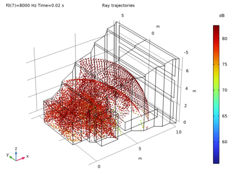
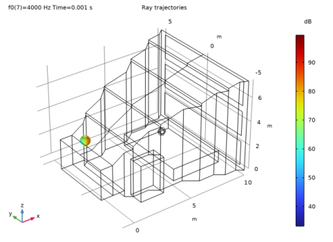
|
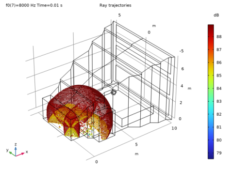
In the Model Builder window, expand the Ray Trajectories (rac) 1 node, then click Ray Trajectories 1.
|
|
2
|
|
3
|
|
4
|
|
1
|
|
2
|
|
3
|
|
4
|
|
1
|
|
2
|
|
3
|
Locate the Data section. From the Dataset list, choose Study 2 - Directional Loudspeaker/Solution 10 (sol10).
|
|
4
|
|
1
|
|
2
|
|
3
|
|
4
|
Locate the Coloring and Style section.
|
|
5
|
|
6
|
|
1
|
|
2
|
|
3
|
|
4
|
|
1
|
|
2
|
|
3
|
Click
|
|
4
|
Browse to the model’s Application Libraries folder and double-click the file small_concert_hall.mphbin.
|
|
5
|
Click
|
|
6
|
|
1
|
|
2
|
On the object imp1, select Boundary 40 only.
|
|
1
|
|
2
|
On the object del1, select Boundary 39 only.
|
|
3
|
|
4
|
Select the Reverse direction checkbox.
|
|
5
|
Click
|
|
1
|
|
2
|
On the object ext1, select Boundary 41 only.
|
|
1
|
|
2
|
|
3
|
|
4
|
On the object del2, select Boundaries 63–65 only.
|
|
1
|
|
2
|
|
3
|
|
4
|
On the object del2, select Boundaries 39–42 and 59 only.
|
|
1
|
|
2
|
|
3
|
|
4
|
On the object del2, select Boundaries 13, 15, 29, 30, 43, 44, 51, and 52 only.
|
|
1
|
|
2
|
|
3
|
|
4
|
On the object del2, select Boundaries 3, 8, 12, 14, 18, and 21 only.
|
|
1
|
|
2
|
|
3
|
|
4
|
On the object del2, select Boundaries 16, 19, 20, 23, 31, and 32 only.
|
|
1
|
|
2
|
|
3
|
|
4
|
On the object del2, select Boundaries 1, 2, 4–7, 9–11, 17, 22, 24–28, 34–37, 45–50, 53–58, and 60–62 only.
|
|
1
|
|
2
|
|
3
|
|
4
|
On the object del2, select Boundaries 33 and 38 only.
|
|
1
|
|
2
|