The coupled damage–plasticity model combines damage mechanics with a plasticity model to describe important characteristics of the mechanical response and failure of concrete and similar materials subjected to multiaxial and cyclic loading conditions. Specifically, it implements the constitutive model for concrete suggested in Ref. 79 and Ref. 80.

The general constitutive equations for the coupled damage–plasticity model uses the concept of the damaged stress tensor σd and the undamaged stress tensor σun. The former is used in the weak formulation while the latter describe the behavior of the intact material.

where σun is split into a positive and negative part by a spectral decomposition in order to account for the anisotropic behavior of concrete in tension and compression. For the same reason, two damage variables introduced: the tensile damage variable dt and the compressive damage variable dc. These variables introduce a weakening of the material’s stiffness, and varies from 0 for an undamaged state to 1 for a fully damaged state. Their definitions are described in Damage Model.

Assuming an additive decomposition of strains, the behavior of the intact material is commonly described by a linear elastic material, such that Hooke’s law relates σun to the elastic strain tensor

where, C is the fourth order elasticity tensor, “:” stands for the double-dot tensor product (or double contraction). The elastic strain εel is the difference between the total strain ε and inelastic strains εinel. The coupled damage–plasticity model always adds a plastic strain tensor εpl to εinel, but other contributions such as thermal strains can also be considered. There may also be an external stress contribution σex, with contributions from initial, viscoelastic, or other inelastic stresses. See also Inelastic Strain Contributions.

The evolution of the plastic deformation is based on the undamaged stress, and thus is independent of damage. A flow plasticity model with isotropic hardening is used , it introduces a yield function Fp, a plastic potential Qp, a scalar hardening variable κp, and the plastic multiplier λp. See also The Plasticity Problem for a general description of how plasticity is solved in COMSOL Multiphysics.

The model can be summarized by the following evolution equations for the plastic strains εpl and the hardening variable κp

The yield function uses a generalization of Willam–Warnke Criterion written as a function of the hardening variable and κp, and the undamaged stress given in the Haigh–Westergaard Coordinates (ξun, run, θun)

here, qh1(κp) and qh2(κp) are hardening functions, and σcs is the uniaxial compressive strength. The friction parameter m0 is written as

where σts is the uniaxial tensile strength and e is the eccentricity parameter.

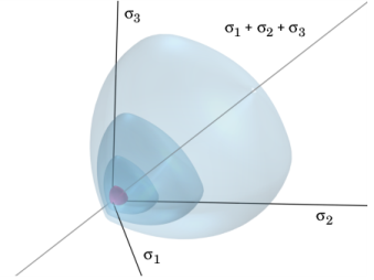
The meridians of the yield surface Fp on the Meridional Plane are parabolic, while the section on the Octahedral Plane is triangular at low confinement and changes toward a circular shape at high confinement. The shape of the section is given by a dimensionless function of the undamaged Lode angle θun

As suggested in Ref. 79 and Ref. 80, the eccentricity is computed as

where σbc is the biaxial compressive strength.

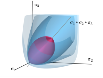
A graphical representation of yield surface Fp = 0 in the undamaged principal stress space and its evolution after hardening is shown in Figure 3-25 and Figure 3-26.

The plastic flow is determined by a nonassociated flow rule, since an associated flow rule typically leads to an overestimation of the concrete strength due to an unrealistically large volume expansion. Here the plastic potential is a simplified version of the yield function in that it is independent of the undamaged Lode angle θun,

where Aq(κp) and Bq(κp) are auxiliary functions derived from the plastic flow in the post-peak regime, see Ref. 80. The functions are defined as

where Df is a model parameter that controls the dilatancy of the plastic flow. By default its value reads Df = 0.85.

The plastic potential in Equation 3-115 leads to a singularity at the point where the plastic potential intersects the hydrostatic axis. Such formulations are not suitable for a numerical implementation. To overcome this, COMSOL Multiphysics modifies Equation 3-115 such that

where J2 is the second invariant of the undamaged stress tensor. The smoothing parameter σv,off controls the distance between where the potential in Equation 3-115 and the smooth potential intersects the hydrostatic axis as exemplified in Figure 3-18 for Drucker–Prager criterion. The parameter σv,off can be estimated as a fraction of the uniaxial compressive strength σcs.

Isotropic hardening controls the evolution of the yield surface during plastic flow. The evolution of the scalar hardening variable κp is proportional to the norm of the plastic strain tensor and follows the evolution equation

The rate of κp depends on the direction of loading such that it grows faster in uniaxial compression, while it is constant in uniaxial tension. The rate of κp is, furthermore, scaled by a ductility measure

such that the material is more ductile in compression. Here Ah, Bh, Ch, and Dh are model parameters, and

COMSOL Multiphysics uses default suggestions for these parameters according to the suggestions given in Ref. 79, where also a calibration procedure from measured data is outlined.

The hardening variable κp enters the two hardening functions qh1 and qh2 that appear in Equation 3-114 and Equation 3-115. These functions control the evolution of the size and shape of the yield function and the plastic potential. They are defined as

where qh0 defines the initial yield limit, and Hp is a dimensionless hardening modulus that controls the hardening in the post-peak regime. Both parameters should be positive and fulfill the inequality Hp + qh0 < 1.

The definition of the two damage variables, dt and dc, are defined in the framework of isotropic damage mechanics, It can described by a damage loading function Fdi and Kuhn–Tucker loading-unloading conditions

where the index i = t, c stands for tension or compression, respectively. In Equation 3-116, εeq stands for the equivalent strain and κdi is a history variable.

where κdi1 and κdi2 are additional history variables.

The equivalent strain is the same for both tension and compression, and it is derived from the plastic yield surface Fp = 0. Using qh1 = 1 and qh2 = εeq / ε0 one can derive

where ε0 = σts / E. Noteworthy is that the equivalent strain εeq reduces to

or directly as εeqt = εeq. The definition of κdt then follows from Equation 3-116 and Equation 3-117.

Two additional history variables, κdt1 and κdt2, are introduced to account for how damage evolves during different stress states. The variable κdt1 is a function of the rate of the plastic strain tensor and it is given by the evolution equation

The variable κdt2 is a function of κdt given by

The evolution of these variables, and thus also the softening response of the model, is sensitive to the multiaxial stress state that enters in the equations through the ductility measure χs. The ductility is defined as

In uniaxial compression, the variables read Rs = 1 and χs = As, which can be useful for calibrating the parameter As. COMSOL Multiphysics by default uses As = 10.

The definition of the history variable κdc then follows after Equation 3-116 and Equation 3-117. The two additional history variables κdc1 and κdc2 are introduced to account for damage evolution at different stress states. The variable κdc1 is a function of the rate of the plastic strain tensor,

and the variable κdc2 is a function of κdt given by

The factor αc is introduced to distinguish between tensile and compressive stresses, and follows from the spectral decomposition of the undamaged stress σun as

where σun,i is the ith principal value of σun, and the operator <  · > denotes the Macaulay brackets. Note that αc varies from 0 in pure tension to 1 in pure compression.

The factor βc is introduced to accomplish a smooth transition between the case of pure damage to damage–plasticity softening, which may occur during cyclic loading. It is defined as

where Df is the same model parameter used for the plasticity flow. The ductility measure χs is defined in Equation 3-118.

Given the history variables, the definition of the damage variables dt and dc follows the same derivation. Assuming monotonic and uniaxial loading, the damaged stress in the softening regime is described by an enhanced inelastic strain, εinel,d,

where fs(·) is the softening law often referred to as the traction–separation law, here given in a terms of inelastic strains.

Since damage is an irreversible process, it is postulated that the inelastic strain εinel,d can be described by the damage history variables. This strain measure is called the inelastic damage strain (or crack-opening strain) and it is defined as

Replacing ε – εinel in Equation 3-119 with κd such that

and using it together with Equation 3-120 results in an equation for the damage variable in terms of the history variables of the form

This nonlinear equation is solved for d using Newton’s method at each material point. COMSOL Multiphysics provides a number of built-in softening functions fs(·) for both tension and compression:

These are depicted in a Figure 3-27. The linear and bilinear definitions have a closed-form solution to Equation 3-121, which makes them computationally attractive.

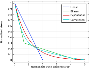
When combined with the crack-band method, the stress versus strain curves in Figure 3-27 are defined in terms of stress versus displacement. The stress versus displacement curves are then converted to unique stress versus strains curves at each material point using the crack-band width hcb, see The Crack Band Method.

In addition to the built-in softening laws, COMSOL Multiphysics allows user-defined definitions of fs(·). Use the variables <phys>.<feat>.<feat>.edmgt and <phys>.<feat>.<feat>.edmgc to defined the damaged strain in tension and compression, respectively. The user-defined function should resemble that in Figure 3-27 with stress and strain interpreted as positive variables in tension and compression.

Alternatively, the user-defined softening behavior can be specified in terms of a stress versus displacement curve, fw(·). Equation 3-121 is then replaced by

assuming that the crack-band method is used. COMSOL Multiphysics provides the variables <phys>.<feat>.<feat>.wdmgt and <phys>.<feat>.<feat>.wdmgc for the damaged displacement in tension and compression, respectively. For both options, the nonlinear equation is solved to find d.