Many materials exhibit a distinct elastic regime where deformations are recoverable and path-independent. This elastic behavior can be modeled using a Linear Elastic Material, Nonlinear Elastic Materials, or Hyperelastic Materials models. In elastoplasticity, the elastic regime is constrained by the yield limit in stress space. When stresses exceed this limit, permanent inelastic strains develop, which, unlike elastic strains, remain even after the stresses are removed.

For elastoplastic materials, the emphasis is primarily on models that capture inelastic strains developing independently of loading rate, known as rate-independent plasticity models. This class of models effectively describes many engineering materials, including homogeneous or porous metals at low temperatures, as well as soils.

In contrast, rate-dependent elastoplastic material models, such as creep and viscoplasticity material models, are commonly applied in scenarios involving high temperatures, where a clear yield limit is difficult to define, or under conditions of high loading rates. For more details on these models, refer to Creep and Viscoplasticity.

The elastoplastic constitutive model is a dissipative model that can be formulated within the framework of thermodynamics using internal variables. In plasticity, the internal variables typically include the plastic strain tensor εpl and a set of hardening variables α.

Plastic deformation occurs when the stresses reach a critical value. In a three-dimensional setting, this may be expressed by a scalar yield function Fy.

where σ is the total stress tensor and A is a set of hardening forces. In case of a geometrically nonlinear case, σ is typically identified as the Cauchy stress tensor. The hardening forces depend on the hardening variables α. In many cases there is only a single hardening force, the scalar yield stress σys. The yield function then reads

The elastic domain is defined as the set of stresses for which the yield function Fy is smaller than zero, that is

For stresses in Ωe no plastic deformation occurs. However, for stresses on the boundary of the elastic domain, where Fy = 0, plastic deformation may occur. This boundary is called the yield surface, which is represented by a hypersurface in stress space. It can be defined as

The flow rule defines the evolution of the plastic deformation. The flow rule is defined in terms of a plastic potential Qp, which is given on the same general form as the yield function

The gradient of the plastic potential Qp with respect to the stress tensor σ gives the direction of plastic flow as

For associated plastic flow, the plastic potential equals the yield function, that is

When the plastic potential is different from the yield function, the flow rule is said to be nonassociated.

When an additive decomposition of strains is used, COMSOL Multiphysics characterizes plastic deformation through the plastic strain tensor εpl. The flow rule then describes how εpl evolves. This equation is postulated as

Here, λ is the plastic multiplier, which is a non-negative variable that satisfies the complementarity condition λFy = 0. The latter condition states that plastic flow may only occur when the stress is on the yield surface.

When a multiplicative decomposition of deformation is used, COMSOL Multiphysics characterizes plastic deformation through the plastic right Cauchy–Green tensor Cp, or more precisely its inverse Cp-1. However, the internal variable is the inverse of the (symmetric) plastic stretch tensor, Up-1, such that Cp-1 = Up-2. An exception is when kinematic hardening is included. Then plastic deformation is characterized by the inverse of the (nonsymmetric) plastic deformation tensor, Fp-1. See Kinematic Hardening for details.

In a multiplicative formulation of plasticity (Ref. 90, Ref. 91, and Ref. 92), the plastic flow rule can be written as the Lie derivative of the elastic left Cauchy–Green deformation tensor Bel:

As for the Additive Plastic Flow, λ represents the plastic multiplier, which is a non-negative variable that satisfies the complementarity condition λFy = 0. The latter condition states that plastic flow may only occur when the stress is on the yield surface.

The Lie derivative of Bel is then expressed in terms of the rate of the plastic right Cauchy–Green tensor

By using Equation 3-52 and Equation 3-53, the plastic flow rule is written as (Ref. 91)

Finally, the elastic left Cauchy–Green tensor is expressed in terms of the deformation gradient F and Cp, so Bel = FCp−1FT. The flow rule then reads

The evolution of the hardening variables is described by the hardening rule. Similarly to the flow rule, the hardening rule for a set of hardening variables α is postulated as

Here, Hp(σ, A) is a general hardening modulus that describes how the hardening variables evolve with plastic deformation.

In principle, any number of hardening variables may be considered and different plasticity models in COMSOL Multiphysics may add one or several such variables. However, the most common approach is to use a single hardening variable, typically the equivalent plastic strain εpe. The general hardening law in Equation 3-55 then simplifies to

The equivalent plastic strain εpe is then used to define how the yield stress σys evolves during plastic flow, that is, σys is the thermodynamic force conjugate to εpe. See Isotropic Hardening for more details.

The hardening modulus hp may take different forms, and it can be specified in a user defined expression.

A common assumption follows from the concept of strain hardening, where the definition of a von Mises equivalent strain is used

Another approach is to derive the hardening modulus hp from a potential, analogous to how plastic flow is defined by taking the gradient with respect to its conjugate hardening force. Here, we assume an associated hardening law, such that

Other variables are added when Kinematic Hardening is combined with a plasticity model.

The mathematical definition of the general plasticity problem is completed by specifying a set of loading and unloading conditions. These conditions are often referred to as the Kuhn–Tucker conditions,

As a result of the second and third conditions, it is concluded that during plastic flow, when λ > 0, it is also required that

In other words, it is required that stresses remain on the yield surface. Equation 3-57 is used to determine the value of the plastic multiplier λ during plastic flow.

The general plasticity problem is defined by Equation 3-49, Equation 3-55, and Equation 3-57, with internal variables εpl, α, and λ.

Here, the superscript n+1 indicates a variable evaluated at the current parameter or time step, and a superscript n denotes a variable with values form the previously converged step.

Also, U represents other dependent variables in the model, such as displacements, that are held fixed within the plastic algorithm, the vector q

is a collection of all plastic variables, and Λ is the incremental plastic multiplier.

For every Gauss point in a domain with an elastoplastic material model, the following algorithm is applied to find the current value of the plastic variables qn+1:

There are additional steps in the algorithm, to ensure that the converged solution fulfills Λ > 0.

It is also possible to specify the maximum number of iterations and the relative tolerance used to solve the plastic algorithm. In the Advanced section of the feature, enter the following settings:

The standard Newton method may not provide a robust solution for highly nonlinear plasticity models. For such models the algorithm can be enhanced by line search iterations in the corrector step (during step d above). This is done automatically for some plasticity models.

In most plasticity features it is also possible to force the use of line search iterations by setting the Local method to Backward Euler, damped. This setting is available in the Advanced section. When selected, it is possible to specify the Maximum number of line search iterations. A common value is 4. It is important to note that an excessive number of line search iterations can cause the algorithm to stall.

When using the multiplicative decomposition, the inverse of the plastic stretch tensor Up-1 is the internal variable used to characterize plastic deformation. In general COMSOL Multiphysics here also applies the so-called exponential mapping technique to discretize the plastic flow rule in Equation 3-54 as

Once the flow rule have been discretized, the numerical solution follows identical steps as described in the Numerical Integration Algorithm section.

The singe yield function in Equation 3-49 is then extended to a set of n yield functions such as

In the general case, the combined yield surface resulting from the set of yield functions is not smooth, and in general, the same applies to the combined plastic potential. Hence, n plastic flow rules are required with corresponding plastic multipliers λi.

COMSOL Multiphysics implements multisurface plasticity models by converting the set of yield functions into a single smooth and C2 differentiable function. This is done by using the procedure outlined in Ref. 115. The same procedure is applied for combining a set of n plastic potentials.

To address this, an iterative approach is employed, where n yield functions are combined into a single smooth function Fysn-1.

Here, s(x) is a smooth function defined as

where a is a smoothing parameter, and g(x) is a function that fulfills certain requirements among them being C2 differentiable. A simple function that meets these requirements is the trigonometric function (Ref. 115)

The smoothing parameter a is then related to the offset of the smooth function Fysn-1 from the nonsmooth function Fy at the intersections of two or more functions Fysk.

from which the plastic dissipation density at the current parameter or time step, Wpn+1, is computed. Here, Λ is the incremental plastic multiplier defined by the Numerical Integration Algorithm.

The total energy dissipated by plasticity in a given volume can be calculated by a volume integration of the plastic dissipation density Wp.

The nonlocal plasticity model implemented in COMSOL Multiphysics is based on the implicit gradient method suggested in Ref. 113, and it incorporates some of the generalizations introduced by the micromorphic theory (Ref. 114).

The theory assumes that the free energy of the elastoplastic material depends on both the macroscopic displacement u and other macrostate variables, such as the equivalent plastic strain εpe, and also on some microstate variable.

When the microstate variable is identified as a nonlocal version of the equivalent plastic strain, εpe,nl, the free energy potential is written as

where Ws is the elastic free energy, Hnl is a model parameter that determines the strength of the coupling between the macro and micro states, and lint is the length scale that determines the influence radius of the interaction.

For simplicity, Equation 3-91 assumes linear isotropic hardening, but the same concept is applicable for more general hardening laws, and it can also be extended to kinematic hardening.

Taking the variation of Equation 3-91 with respect to the state variables εpe, εpe,nl, and ∇εpe,nl leads to the following set of equations related to the plasticity model:

here, Ω represents the domain of the elastoplastic problem.

The variation of Equation 3-91 with respect to the remaining state variables leads to the standard elasticity equations. In the nonlocal (or regularized) plasticity problem, εpe,nl is an additional dependent variable that is solved as part of the global problem.

The structure of the local plasticity problem is not changed, and the numerical solution remains the same as discussed for the Numerical Integration Algorithm. The only difference is that the hardening force σys now also depends on εpe,nl.

Add a Set Variables subnode to Metal Plasticity, Porous Plasticity, Pressure-Dependent and Soil Plasticity, or Elastoplastic Soil Models to set up the plastic strain tensor, plastic deformation gradient, the equivalent plastic strain, and other internal variables.

Permanent or plastic deformations in metals and other ductile materials is generally assumed to appear when the maximum shear stress or some other measure of distortion exceeds a critical value. This means that plastic yielding is independent of the hydrostatic pressure. Such models are often referred to as volume preserving plasticity models. The yield function is commonly described by the classical von Mises or Tresca criterion, but orthotropic plasticity may also be considered using the Hill criterion.

For a general discussion on plasticity and its implementation in COMSOL Multiphysics, see The Plasticity Problem section.

The von Mises criterion suggests that yielding of the material occurs when the second deviatoric stress invariant J2 reaches a critical value k. Hence, von Mises plasticity is often also referred to as J2 plasticity. It can be written in terms of the elements of Cauchy’s stress tensor (Ref. 51)

where σys is the uniaxial yield stress level and is the equivalent von Mises stress. An associative flow rule is always used for the von Mises criterion, that is, Qp = Fy

The Tresca criterion suggests that yielding occurs when the maximum shear stress reaches a critical value. Given a spectral decomposition of Cauchy’s stress tensor, the maximum shear stress is expressed as

where σ1 is the maximum principal stress and σ3 is the minimum principal stress. The Tresca criterion then reads

where τys is the shear yield stress. Alternatively, it can be expressed using the uniaxial yield stress σys, as for the von Mises criterion, and then reads

where σtresca = σ1 − σ3 is the equivalent Tresca stress.

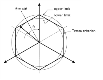
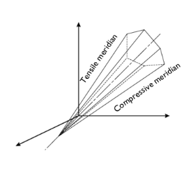
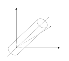
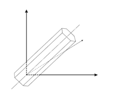
Graphically, the Tresca yield surface is represented by an infinite hexagonal prism in principal stress space with it axis coinciding with the hydrostatic axis, see Figure 3-15. The elastic domain corresponds to the inside of the hexagon. The shape of the hexagonal yield surface can be further visualized by projecting it onto the Octahedral Plane as shown in Figure 3-16. The upper limit in this surface corresponds to the von Mises yield surface.

For the case of associated plastic flow, COMSOL Multiphysics constructs a smooth plastic potential to handle the edges of the hexagonal yield function, by using the procedures outlined in Multisurface Plasticity. In general, a full representation of the hexagon requires six yield functions combined into one. However, since the principal stresses are sorted such that σ1 > σ2 > σ3, it is sufficient to consider three functions only

Note that the exact representation of the yield function in Equation 3-59 is used for the associated plastic flow.

Hill (Ref. 93, Ref. 94) proposed a quadratic yield function given by the principal axes of orthotropy ai in a local coordinate system. The yield function can be written in terms of the elements of Cauchy’s stress tensor as

Here, σ is the vector representation of the stress tensor in Voigt order, see Orthotropic and Anisotropic Materials. The symmetric 6-by-6 matrix reads

where the parameters F, G, H, L, M, and N are related to the state of anisotropy.

To write the Hill criterion in a similar way as done for the von Mises and Tresca criteria, an average initial yield stress σys0 is defined from the parameters F, G, and H as

with σys = σys0 if there is no isotropic hardening.

The parameters of the Hill criterion can be related to the initial yield stresses with respect to the axes of orthotropy ai. The first three parameters are related to the initial uniaxial yield stresses σys1, σys2, and σys3 as

and the remaining three parameters are related to the initial shear yield stresses σys12, σys13, and σys23 as

The yielding of many engineering materials is sensitive to the hydrostatic pressure. Such materials include biological tissue, polymers, foams, clays, and geotechnical materials. Assuming isotropic plastic deformation, the plasticity models for a large class of such materials can be constructed from the Invariants of the Stress Tensor. Here we use the following three invariants:

Here, σm is the mean stress, σmises is the von Mises equivalent stress, and θ is the Lode angle.

The Pressure-Dependent Plasticity and Soil Plasticity features implement a number of plasticity models that can be described by a yield function of either a parabolic form

Here, Γ(θ) is a function of the Lode angle θ that defines the shape of the yield function in the Octahedral Plane. The most common choice, Γ(θ) = 1, results in a circular section. Similarly, Ma(σm) and Mb(σm) are functions of the mean stress σm that define the shape of the yield function in the Meridional Plane.

The yield stress σys is here interpreted as the stress level when yielding occurs given Γ(θ) = 1 and σm = 0. Various Isotropic Hardening models can be added by specifying the yield stress σys as a function of the equivalent plastic strain εpe.

The Drucker–Prager criterion is as an extension of the von Mises Criterion to include pressure-dependence. It is available in both the Pressure-Dependent Plasticity and Soil Plasticity features and it can be used to model a wide variety of materials.

The resulting yield function is the simplest specialization of Equation 3-60, where Γ(θ) = 1 and Ma(σm) = a1σm. The yield function reads

where a1 is a model parameter that controls the pressure dependence. In this expression, the mean stress σm corresponds to the negative pressure, that is, it is positive in tension.

The parameter a1Q controls the influence of pressure on the plastic flow.

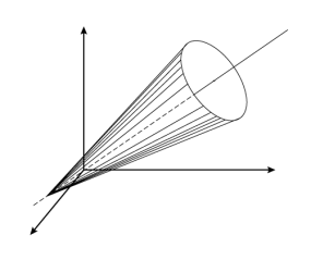
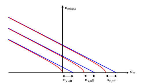
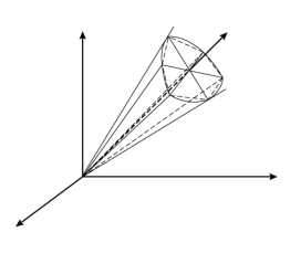
The plastic potential in Equation 3-62 leads to a singularity in the flow rule where the yield surface intersects the hydrostatic axis, that is, the tip of the cone. Such formulation is not suitable for a numerical implementation. To handle this, COMSOL Multiphysics modifies Equation 3-62 such that a smooth plastic potential is obtained with a rounded vertex. The smooth plastic potential is written as

Here, the smoothing parameter σv,off controls the distance where the potential in Equation 3-62 and the smooth potential in Equation 3-63 intersect the hydrostatic axis as shown in Figure 3-18.

For Soil Plasticity, the parameters in Drucker–Prager criterion receive different names to comply with geotechnical conventions. The yield function is written as

The parameters k, α, and αQ are generally identified from common soil parameters: cohesion c; friction angle ϕ; and dilatation angle ψ, and by matching the Drucker–Prager criterion to the Mohr–Coulomb Criterion. This can be done using different assumptions:

The elliptic criterion in Pressure-Dependent Plasticity implements Equation 3-61 with the meridional shape function parameterized with a linear and a quadratic dependence on the mean stress σm as

The shape of the yield function in the Octahedral Plane is generally circular, but it can be made a function of the Lode angle θ by using any of the functions described in Octahedral Section.

Setting b1 = 0 recovers an ellipse like in for example the Cam–Clay family of models. Parameter b3 > 0 then represents the shift of the ellipse along the hydrostatic axis, and parameter b2 gives the aspect ratio of the ellipse in the Meridional Plane.

Setting b2 = 0 and b1 > 0 results into a paraboloid that opens into the compressive direction and intersects the hydrostatic axis at σm = σys2/b1. Setting b1 = 0 and b2 = 0 recovers the von Mises Criterion.

with a set of three parameters to control the shape of the plastic potential in the Meridional Plane. For nonassociated flow, the plastic potential is always assumed to be independent of the Lode angle θ, and its projection on the Octahedral Plane is thus circular.

The parabolic criterion in Pressure-Dependent Plasticity implements Equation 3-60 with the meridional shape function parameterized with a linear, a quadratic, and an exponential dependency on the mean stress σm as

The shape of the yield function in the Octahedral Plane is generally circular, but it can be made as a function of the Lode angle θ by using any of the functions described in Octahedral Section.

Setting a1 > 0, a2 = a3 = 0 recovers the Drucker–Prager criterion. By setting a2 > 0, a1 = a3 = 0, a closed parabola is obtained similar to, for example, the GAZT criterion for foams.

with a set of four parameters to control the shape of the plastic potential in the Meridional Plane. For nonassociated flow, the plastic potential is always assumed to be independent of the Lode angle θ, and its projection onto the Octahedral Plane is thus circular.

The plastic potential in Equation 3-64 leads to a singularity in the flow rule where the yield surface intersects the hydrostatic axis, that is, the vertex of the cone. This formulation is not suitable for a numerical implementation. To handle this, COMSOL Multiphysics modifies Equation 3-64 such that a smooth plastic potential with a rounded vertex is used. The smooth plastic potential is written as

Here, the smoothing parameter σv,off controls the distance between where the potential in Equation 3-64 and the potential in Equation 3-65 intersect the hydrostatic axis. If α1Q = 0, a small fall-back value is used in the square root term of Equation 3-65. The smooth plastic potential is used for the associated plastic flow also.

The profile of the yield function on the Octahedral Plane is useful for denoting changes in the yield limit under different loading conditions, for example, compression or tension. COMSOL Multiphysics provides three alternative definitions of the function Γ(θ) that controls the shape of the yield function on the octahedral plane:

Gudehus (Ref. 96) proposed an octahedral section that changes with the Lode angle θ. The change in the cross sectional shape depends on one parameter as

A value of c = 1 represents a circular section. Independent of the value of the parameter c, the function equals at the tensile meridian (θ = 0), and at the compressive meridian. For c < 1, the tensile strength is lower than the compressive strength. The function Γ(θ) is thus an approximation of the ratio of tensile to compressive strength. For the function to be convex, the parameter c has a lower bound of 7/9 and an upper bound of 9/7.

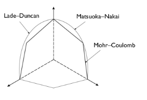
Panteghini and Lagioia (Ref. 97) proposed a three-parameter function to control the octahedral section based on the Lode angle as follows:

The function was derived with the purpose to recover common soil plasticity yield functions, including a rounded Mohr–Coulomb Criterion, the Matsuoka–Nakai Criterion, and the Lade–Duncan Criterion. However, the three parameters of the function provide a flexible option to control the octahedral section in a general manner. Setting the parameter c2 < 1 creates a continuous and C2 differentiable function.

The foam plasticity model in Pressure-dependent plasticity, is an elliptic model that is a generalization of the model first proposed by Deshpande and Fleck (Ref. 116) to model structural foams. It is popular not only for modeling the failure of metallic foams, but also for battery cells, biological tissue, and other materials with a cellular structure.

The COMSOL Multiphysics implementation of the model can be seen as a specialization of Equation 3-61 with the yield function written as

The shape of the ellipse is controlled by three parameters, where pt and pc define the limits in hydrostatic tension and compression, respectively. The parameter α controls the aspect ratio of the ellipse, and it is inferred from the initial uniaxial compressive strength σuc0 such that

Here, pc0 is the initial yield stress in hydrostatic compression when hardening is considered, which means that the aspect ratio of the ellipse is constant after plastic deformation.

Compared to the yield function in Equation 3-68, the centroid of the ellipse defined by the plastic potential in Equation 3-69 is located at the origin of the Meridional Plane. The shape of the plastic potential is defined by a single parameter, β, that controls the aspect ratio of the ellipse. The parameter is defined by the plastic Poisson’s ratio νp as

The plastic Poisson’s ratio is identified as the ratio of longitudinal to transverse plastic strain, and has a lower limit of -1 and an upper limit of 0.5. A common assumption for metallic foams is νp = 0, which results in a parameter β = 9/2.

The foam plasticity model is intended to model the compaction of materials and thus adds a volumetric hardening model. The hardening rule is implemented for the evolution of the internal plastic variable εpv, which is the equivalent volumetric plastic strain. The hardening rule is set up so that εpv is monotonically increasing and it only accounts for the compaction of the material

Note that εpv is positive in compression.

where pch is a hardening function. A common hardening model for foams is that the compressive yield stress varies with the volumetric strain by a power function, that is, pch(εpv) =  C εpvn.

Test data is sometimes more commonly available in terms uniaxial compressive stress and strain. COMSOL Multiphysics then also provides the option to specify hardening data in terms of the uniaxial compressive strength σuc and the axial equivalent plastic strain εpa as

The axial equivalent plastic strain εpa is difficult to identity for general loading conditions. It is therefore estimated from the equivalent volumetric plastic strains εpv and the plastic Poisson’s ratio νp as

Note that when volumetric hardening is included, it is only the yield stress in hydrostatic compression pc that evolves with the plastic deformation. All other parameters that define the yield function and plastic potential remain fixed.

The Mohr–Coulomb criterion is a classical and popular criterion in soil mechanics. It was developed by Coulomb before the Tresca and von Mises criteria for Metal Plasticity, and it was the first criterion to include the hydrostatic pressure. The criterion states that failure occurs when the shear stress and the normal stress acting on any element in the material satisfy the equation

were, τ is the shear stress, c the cohesion, and ϕ denotes the friction angle.

The Mohr–Coulomb criterion can be written in terms of invariants as a specialization of the general yield function presented in Equation 3-60. Since the yield function has a hexagonal octahedral section, it is written as

Here parameters α and k are defined by the friction angle ϕ and the cohesion c as

To define an octahedral section that equals the hexagonal shape of the Mohr–Coulomb criterion, the function in Equation 3-67 is used. To define the Mohr–Coulomb yield function, the three parameters of Equation 3-67 are defined as

The choice of these parameters results in the hexagonal pyramid depicted in Figure 3-19 with the sharp corners. If used as plastic potential for the flow rule, this leads to singularities and a formulation not suitable for a numerical implementation. COMSOL Multiphysics defines the smooth plastic potential as

where the vertex is rounded using the same method as for the Drucker–Prager Criterion. The sharp corners of the octahedral section are rounded by setting c2 = β with β < 1 for the plastic potential. This results in a smooth and continuous octahedral section that inscribes the Mohr–Coulomb criterion. The default value is β = 0.99. Setting a lower value for β increases the radius of the rounded corners.

The Mohr–Coulomb criterion can be used with either an associated or nonassociated flow rule. For the associated flow rule, αQ = α such that the pressure dependence of plastic flow is governed by the friction angle ϕ. When a nonassociated flow rule is used, αQ is defined by the dilatation angle ψ as

It is also possible to use a simplified flow rule with the plastic potential defined by Equation 3-63, that is, independent of the Lode angle θ.

Matsuoka and Nakai (Ref. 55) discovered that the sliding of soil particles occurs in the plane in which the ratio of shear stress to normal stress has its maximum value, which they called the mobilized plane. The yield surface is based on the first, second, and third Invariants of the Stress Tensor as

where the parameter μ = (τ/σn)STP equals the maximum ratio between shear stress and normal stress in the spatially mobilized plane (STP-plane). The invariants are applied over the effective stress tensor, this is, the stress tensor minus the fluid pore pressure.

The Matsuoka–Nakai criterion circumscribes the Mohr–Coulomb Criterion when the parameter μ equals

where ϕ denotes the friction angle.

As shown in Ref. 97, the above formulation of the Matsuoka–Nakai criterion is not suitable for numerical implementation since it results in false elastic domains in the tensile octant’s of the principal stress space.

COMSOL Multiphysics implements the Matsuoka–Nakai criterion as a specialization of the general yield function presented in Equation 3-60. Since the yield function has a noncircular octahedral section, it is written as

Here, the parameters α and k can be defined by the friction angle ϕ and the cohesion c as

To define an octahedral section that equals the Matsuoka–Nakai criterion, the function proposed by Panteghini and Lagioia (Ref. 97) in Equation 3-67 is used. Here, the three parameters of Equation 3-67 are defined as

As for all parabolic yield functions, the Matsuoka–Nakai yield function has a singularity where it intersects the hydrostatic axis. Therefore, the same smooth plastic potential as for the Mohr–Coulomb criterion (Equation 3-70) is used.

The Matsuoka–Nakai criterion can be used with either an associated or nonassociated flow rule. For the associated flow rule, αQ = α, such that the pressure dependence of plastic flow is governed by the friction angle ϕ. When a nonassociated flow rule is used, αQ is defined by the dilatation angle ψ as

It is also possible to use a simplified flow rule with the plastic potential defined by Equation 3-63, that is, independent of the Lode angle θ.

where I1 and I3 are the first and third Invariants of the Stress Tensor, respectively, and kLD is a parameter related to the direction of the plastic strain increment in the triaxial plane. It can be derived from the friction angle ϕ as

The Lade–Duncan criterion does not match the Mohr–Coulomb Criterion at the tensile meridian (θ = 0).

As shown in Ref. 97, the above formulation of the Lade–Duncan criterion is not suitable for numerical implementation since it results in false elastic domains in the tensile octants of the principal stress space.

COMSOL Multiphysics instead implements Lade–Duncan criterion as a specialization of the general yield function presented in Equation 3-60. Since the yield function has a noncircular octahedral section, it is written as

Here, parameters α and k can be defined by the friction angle ϕ and the cohesion c as

To match an octahedral section corresponding to Lade–Duncan criterion, the function proposed by Panteghini and Lagioia (Ref. 97) is used. Here, the three parameters of Equation 3-67 are defined as

As for all parabolic yield functions, the Lade–Duncan yield function has a singularity where it intersects the hydrostatic axis. Therefore, the same smooth plastic potential as for the Mohr–Coulomb criterion (Equation 3-70) is used.

The Lade–Duncan criterion can be used with either an associated or nonassociated flow rule. For the associated flow rule, αQ = α, such that the pressure dependence of plastic flow is governed by the friction angle ϕ. When a nonassociated flow rule is used, αQ is defined by the dilatation angle ψ as

It is also possible to use a simplified flow rule with the plastic potential defined by Equation 3-63, that is, independent of the Lode angle θ.

For any parabolic type plasticity models, a cap can be added to the plasticity model to limit the elastic domain in compression. This is of particular interest for models that are linear in the Meridional Plane such as the Drucker–Prager Criterion, and other soil plasticity models where the yield function opens in the compressive direction of the hydrostatic axis. Normally, these models are not accurate above a given pressure limit, since real-life materials cannot bear infinite loads and still behave elastically. To circumvent this, two types of cap models can be added in COMSOL Multiphysics

The elliptic cap formulation is the most comprehensive, often providing more accurate predictions of observed behavior. However, the simplicity of the planar cap makes it a practical alternative in some cases. Both formulations employ an associated flow rule and allow for hardening that is independent of the yield functions.

The combination of a general parabolic yield function with either cap formulation leads to an unsmoothed yield surface, which is unsuitable for numerical implementation. To overcome this, COMSOL Multiphysics uses the procedures outlined in Multisurface Plasticity to construct a smooth and C2 differentiable yield surface.

The yield function of the planar cap only depends on the mean stress σm

where pc is the pressure limit. The yield function imposes a pressure limit that restricts any values exceeding pc.

where pc0 is the initial pressure limit, and pch is the hardening function that depends on the hardening variable εpc. A perfectly plastic model assumes pch = 0.

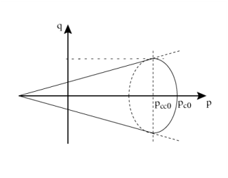
The yield function of the elliptic cap is a function of stress invariants σm, σmises, and θ; it only depends on the Lode angle if the parent yield function does. For the most general case, the yield function reads

Where the operator <  · > represents the Macaulay brackets. The term Fy(−pcc,0,0) implies that the parent yield function is evaluated at σm = −pcc, and at zero von Mises stress and zero Lode angle, σmises = θ = 0.

The location and the shape of the ellipse is controlled by its centroid on the hydrostatic axis, pcc, and its aspect ratio R. The latter is defined by

where pc0 is the initial pressure limit and pcc0 is the initial location of the centroid on the hydrostatic axis. This definition implies that the aspect ratio is constant also when hardening is included.

Figure 3-22 visualizes the combined yield surface of a Drucker–Prager yield function and the elliptic cap with no hardening on the meridional plane.

Here pcch is the hardening function that depends on the hardening variable εpc. However, when the Drucker–Prager Criterion is used, the hardening model directly specifies the evolution of the pressure limit pc as

where pc0 is the initial pressure limit and pch is the hardening function. The current value of the centroid variable, pcc, is then computed from pc using geometrical considerations.

The variable εpc is an internal plastic variable added when hardening is included. The additional hardening rule for this variable reads

where hc is the hardening modulus.

The hardening modulus is often defined as the rate of the volumetric plastic strain, that is the trace of the Plastic Flow Rule, hc = tr Gpl, but it can also be defined as a user defined expression.

The condition in Equation 3-71 means that the hardening variable εpc decreases monotonically with volumetric plastic deformation. However, it is possible to allow the cap to soften. The cap is then limited to move along the compressive part of the hydrostatic axis, and the hardening rule is modified to read

When applying hardening to the planar cap, the variable for the centroid of the ellipse, pcc, is replaced by the variable for the pressure limit, pc.

The hardening functions pch and pcch can be defined by user defined expressions. COMSOL Multiphysics also includes built-in hardening functions intended to model an exponential variation of the material density during compaction.

for the elliptic cap. For both formulations, Kc is the hardening modulus and is the maximum volumetric plastic strain.

In general, the Rankine cutoff offers a more accurate formulation, whereas the mean stress cutoff provides a more efficient and robust alternative. Both cutoff models utilize an associative flow rule. However, combining a general parabolic yield function with either cutoff formulation leads to an non-smooth yield surface, which is unsuitable for numerical implementation. To overcome this drawback, COMSOL Multiphysics uses the procedures outlined in Multisurface Plasticity to construct a smooth and C2 differentiable yield function.

The yield function of the mean stress cutoff is only dependent on the mean stress σm and reads

where σm,t is the mean stress limit in tension. The yield function implies that a mean stress exceeding σm,t is not allowed.

The Rankine criterion states that the maximum principal stress cannot exceed the tensile strength σts. Since COMSOL Multiphysics sorts the principal stresses (σ1 > σ2 > σ3), the criterion reads

and the applies the procedures outlined in Multisurface Plasticity to construct a smooth and C2 differentiable yield function Fcutoff.

A plasticity model with isotropic hardening is characterized by a yield surface that expands (or shrinks) uniformly during plastic deformation. For example, for the von Mises Criterion furbished with an isotropic hardening law implies that the radius of the cylinder in stress space changes during plastic deformation, but its axis remain on the hydrostatic axis.

An isotropic hardening model typically considers a single scalar hardening variable. COMSOL Multiphysics uses the equivalent plastic strain εpe as described by the hardening rule in Equation 3-56. By default, most plasticity features assume a strain hardening approach to define εpe, but other definitions may also be considered.

Isotropic hardening is added to a the general yield function in Equation 3-50 by letting the yield stress σys be a function of the equivalent plastic strain εpe. That is, the yield functions reads

where σe is the scalar equivalent stress. COMSOL Multiphysics provides several types of isotropic hardening models for elastoplastic materials:

Here the yield stress is given by the initial yield stress σys0 such that it is constant and independent on the equivalent plastic strain variable εpe

The yield stress σys(εpe) is for linear isotropic hardening a function of the equivalent plastic strain εpe and the initial yield stress σys0

Here, the isotropic hardening modulus Eiso is derived from

For linear isotropic hardening, the isotropic tangent modulus ETiso is defined as (stress increment / total strain increment). The Young’s modulus E is taken from the parent material model. If the elasticity of the parent material is anisotropic or orthotropic, E represents an equivalent Young’s modulus.

In the Ludwik model for nonlinear isotropic hardening, the yield stress σys(εpe) is defined by a nonlinear function of the equivalent plastic strain. The Ludwik equation (also called the Ludwik–Hollomon equation) for isotropic hardening is given by the power law

Here, k is the strength coefficient and n is the hardening exponent. Setting n = 1 would result in linear isotropic hardening.

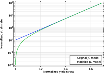
Similar to the Ludwik hardening model, the yield stress σys(εpe) is in the Johnson–Cook model defined as a nonlinear function of the equivalent plastic strain εpe given by a power law. The difference is that effects of the strain rate are included in the model. The yield stress and hardening function is given by

The Johnson–Cook model also adds the possibility to include thermal softening by including a function which depends on the normalized homologous temperature Th. It is a function of the current temperature T, the melting temperature of the metal Tm, and a reference temperature Tref

As a default, this dependency follows a power law, . The softening function f(Th) should have the properties f(Th < 0) = 0 and f(Th> 1) = 1.

The strain rate strength coefficient C and the reference strain rate in the Johnson–Cook model are obtained from experimental data. The flow curve properties are normally investigated by conducting uniaxial tension tests in a temperature range around half of the melting temperature Tm, and subjected to different strain rates like 0.1/s, 1/s, and 10/s.

The original motivation of the Johnson–Cook is to model material failure at high strain rates, and it can be shown that the strain rate dependent term in Equation 3-72 is only valid when . The implementation of the Johnson–Cook model in COMSOL Multiphysics thus reads

where the operator <  · > represents the Macaulay brackets, such that the logarithmic function never evaluates to a negative number. In this formulation, the reference strain rate must be considered in the quasistatic limit. Below this value, the hardening function will be strain rate independent, but temperature dependent, similar to Ludwik law:

an alternative implementation is provided for the case when hardening must account for both high and low strain rates, possibly in the same material point as the loading changes. This yield stress for this modified Johnson–Cook model is given by

which is valid for . At high strain rates where it approaches the original model in Equation 3-72, while for the strain rate dependence becomes similar to Peric Model.

For nonsaturating materials, the Swift power law equation relates the initial yield stress σys0 and the isotropic hardening σh, to the equivalent plastic strain as

here, k is the strength coefficient, n is the hardening exponent, and ε0 is a reference strain. Noting that at zero plastic strain the initial yield stress is related to the strength coefficient and hardening exponent as

The Voce function for nonlinear isotropic hardening is intended for materials that exhibit a saturating evolution of hardening. The isotropic hardening σh is exponentially related to the equivalent plastic strain as

The yield stress σys(εpe) is then defined as

The value of the saturation exponent parameter β determines the saturation rate of the hysteresis loop for cyclic loading. The saturation flow stress σsat characterizes the maximum distance by which the yield surface can expand in the stress space. For values εpe >> 1/β, the yield stress saturates to

where σ∝ is the steady-state flow stress, m the saturation coefficient and n the saturation exponent. For values mεpen >> 1 the yield stress saturates to

In this case, define the (usually nonlinear) hardening function σh(εpe) such that the yields stress reads

A plasticity model with kinematic hardening is characterized by a yield surface that translates during plastic deformation, keeping its initial shape. For example, for the von Mises Criterion adding a kinematic hardening law implies that the radius of the cylinder in stress space is constant, but its axis deviates form the hydrostatic axis.

Many engineering materials, particularly metals, exhibit the Bauschinger effect. This phenomenon occurs when a specimen is first loaded in tension until yielding, then unloaded and reloaded in compression. The compressive yield stress is observed to be lower than if the material had been initially loaded in compression. The Bauschinger effect is commonly explained by kinematic hardening, which is one of the primary motivations for incorporating this hardening mechanism in material models.

A kinematic hardening model can be incorporated into the general yield function in Equation 3-50 by shifting the stress tensor σ by the so-called back stress σb. The yield function then reads

where σe is the scalar equivalent stress. There are three built-in models to define the evolution of the back stress during plastic deformation:

The models are described with the assumption of an additive decomposition of strains and then for a Multiplicative Decomposition.

In the linear kinematic hardening model, also known as Prager’s hardening rule, the evolution the back stress is selected as the hardening variable. The hardening rule is written such that the evolution of the back stress is proportional to the rate of the plastic strain tensor εpl

COMSOL Multiphysics assume that the kinematic hardening modulus Ck is constant, in which case no additional equation is solved, and the back stress σb is defined directly from the plastic strain tensor

That is, the model does not add additional internal variables. The kinematic hardening modulus Ck is given by

where Ek is the kinematic tangent modulus and the Young’s modulus E is taken from the parent material model. If the elasticity of the parent material is anisotropic or orthotropic, E represents an equivalent Young’s modulus.

Armstrong and Frederick (Ref. 88) proposed an extension to Prager’s linear kinematic hardening model, by introducing additional terms to Equation 3-73

here, γk is a model parameter, Ck is the kinematic hardening modulus, and λ is the plastic multiplier. The additional term introduces an effect of saturation in the hardening rule.

The implementation of the Armstrong–Frederick model in COMSOL Multiphysics uses a back strain tensor εb as the hardening variable. The relation between εb and the back stress is

Considering this relation, Equation 3-74 is rewritten so that the hardening rule to define the evolution of the back strain reads

Chaboche (Ref. 89) proposed a nonlinear kinematic hardening model based on the superposition of N back stress tensors

where each of these back stress tensors σb,i follow a nonlinear Armstrong–Frederick kinematic hardening rule

Practitioners would normally select γk = 0 for one of the back stress equations, thus recovering Prager’s linear rule for that branch

The back stress tensor σb is then defined by the superposition of N back stress tensors

As done for the Armstrong–Frederick kinematic hardening, the algorithm solves for the back strain tensors εb,i instead of the back stress tensors σb,i. The change of variables is

and the nonlinear evolution for the back strain tensors in Equation 3-75 reads

For multiplicative decomposition, the total deformation gradient F is decomposed into an elastic Fel and a plastic (inelastic) deformation Fpl

as described in Inelastic Strain Contributions.

When kinematic hardening is used with multiplicative decomposition, Fpl is split as suggested in Ref. 95, such that

Here Fple is referred to as the “elastic” part of Fpl, and Fplv as the “viscous” part of the plastic deformation. Conceptually, Fple corresponds to a spring and Fplv to a dashpot that are connect in series in a rheological model. Also, new kinematic quantities can be defined in a similar fashion as defined for Fel. For example, the tensor

which is analogous to the elastic right Cauchy–Green deformation tensor Cel. As for the elastic part of the model, a free energy function Wkin(Cpl,e) is defined for the spring of the kinematic hardening contribution. Different stress tensors can be derived, for example

which represents that back stress in the material frame and is analogous to the second Piola–Kirchhoff stress of the elastic part. By applying a push-forward operation by the total deformation gradient F, the back stress in the spatial frame is

where is a representation of the back stress in an intermediate frame defined by Fpl. The yield function in Equation 3-63 is defined in the spatial frame for large strains, thus to complete the formulation we need to define σb or Cple, which depends on the kinematic hardening model used.

For linear elastic materials, it is assumed that Wkin has the same form as the elastic strain energy function, and that it is always isotropic. Hence, for a linear elastic material the free energy function Wkin reads

where εple = 0.5(Cple−1) and Ck is the kinematic hardening modulus.

The flow rule suggested for the Multiplicative Decomposition leads to an arbitrary plastic rotation, which is undesirable with the above formulation for kinematic hardening. Hence, when kinematic hardening is used, the plastic flow rule is modified to

To obtain a linear kinematic hardening model the inelastic part of the plastic deformation is omitted by setting Fplv = 1, and thus Cple = Cpl.

To obtain the Armstrong–Frederick kinematic hardening model, the inelastic part of the plastic deformation Fplv is considered as an additional variable determined by the flow rule

where γk is a kinematic hardening parameter. The actual unknown used by the plasticity algorithm is the symmetric part of the inverse of Fplv.

The Chaboche kinematic hardening model can be viewed as a combination of linear kinematic hardening and Armstrong–Frederick kinematic hardening by adding N branches. Formally, each branch corresponds to a unique multiplicative split of Fpl such that for branch i the multiplicative decomposition reads

Conceptually, each branch corresponds to a spring and a dashpot in series, and all the branches are connected in parallel. The first branch always corresponds to linear kinematic hardening such that Fplv,1 = 1. Each consecutive branch adds an Armstrong–Frederick kinematic hardening model, where Fplv,i is an additional variable with its own flow rule. The total back stress is then the sum of the stress in all branches

Both Isotropic Hardening and Kinematic Hardening can be incorporated into the same plasticity model, a formulation known as mixed hardening. These more refined hardening models are often necessary to accurately capture the true behavior of many materials.

The general yield function in Equation 3-50 then reads

where σe is the scalar equivalent stress.