COMSOL 6.3 - Lumped Composite Thermal Barrier with Shells

Lumped Composite Thermal Barrier with Shells

This example shows how to replace two 3D finite element domains by thin structures for heat transfer modeling, and to connect them through a lumped thermal system to account for a thermal barrier.

The model is a variant of the Composite Thermal Barrier and Lumped Composite Thermal Barrier models, in which two ceramic thin layers with different thermal conductivities are sandwiched in a steel column.

Three modeling approaches are compared for the computation of the temperature distribution through the whole column. First, both the steel column and the composite (made of the ceramic layers) are modeled as 3D objects. In the second approach, to avoid resolving both the column and the ceramic layers in the geometry, the Heat Transfer in Shells interface is used to model the upper and lower parts of the steel column, and the Lumped Thermal System interface is used for the ceramic layers, and coupled to the two shells through boundary conditions. Finally, the equivalent lumped system is simulated with a single resistor carrying the equivalent thermal resistance of the ceramic layers. In case of such simple lumped thermal system, it can be entirely encapsulated in the feature, the Lumped Thermal System physics interface is then not required.

This methodology is useful when modeling heat transfer through thermal barriers like multilayer coatings.

Model Definition

Geometry

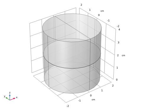
This tutorial uses a simple geometry as shown in Figure 1. The cylinder has a radius of 2 cm and a height of 4 cm.

Figure 1: Geometry.

The composite consists of two layers with different thermal conductivities. The first approach resolves each layer as a 3D domain. The height of the layers is about three orders of magnitude smaller than the bulk height. This often requires to build a mesh manually to accurately resolve the thin structure.

Thin Structure Representation of the Steel Column

The Heat Transfer in Shells interface is used to model the conductive heat transfer in the top and bottom parts of the steel column.

The top and bottom cylinders are represented by two circular shells whose thickness is defined in the settings. Although the column thickness is not represented explicitly in the geometry, the Layered Material technology allows to solve the temperature distribution through the shells. The number of implicit mesh elements can be set in the node as well, to fit the settings used for the swept meshes of the 3D domains.

The condition is applied on the bottom interface of the lower part of the column, and on the top interface of the upper part of the column, to prescribe the temperature at each extremity of the column.

Network Representation of the Thermal Barrier

COMSOL Multiphysics provides the Lumped Thermal System physics interface, available from the Heat Transfer Module, and in which the feature allows to model conductive heat transfer without representing the underlying geometry.

The Lumped Thermal System physics interface uses a network representation of thermal systems to model heat transfer by analogy with electrical circuits. The domain and boundary conditions for heat transfer are idealized by components joined by a network of perfectly thermally conductive wires.

This 0D approach simplifies the geometry and thus the mesh. In complex geometries, this lumped approach can significantly reduce the amount of memory and time required for the simulation.

For the modeling of the thermally resistive ceramic layers, two components are connected in a serial circuit.

The coupling between the two physics interfaces, Heat Transfer in Shells (2D approach) and Lumped Thermal System (0D approach), is performed through the following features:

•

feature in the Heat Transfer in Shells interface, applied on the bottom interface of the top shell, and on the top interface of the bottom shell. This feature uses the heat rate defined by each feature to set a heat flux on the corresponding boundary in the distributed finite element model.

•

feature in the Lumped Thermal System interface, applied at each extremity of the thermal circuit. This feature prescribes the temperature Text provided by the feature of the Heat Transfer in Shells interface.

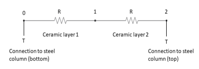
The complete thermal circuit modeled by the Lumped Thermal System interface is as shown in Figure 2.

Figure 2: Thermal circuit for heat transfer in the ceramic layers.

Conductive Thermal Resistor

The feature models heat conduction in a thin shell of constant conductivity. In this example, a plane shell configuration is assumed, and the thermal resistance R (SI unit: K/W) of each layer is expressed from the thermal conductivity k (SI unit: W/(m·K)), the thickness L (SI unit: m), and the surface area A (SI unit: m²) as follows:

It then assumes that the heat rate P (SI unit: W) through each layer is proportional to the temperature difference ΔT (SI unit: K) across it:

See Theory for the Lumped Thermal System Interface in the Heat Transfer Module User’s Guide for more details about the underlying theory.

In case of a lumped thermal system consisting of two serially connected resistors as presented in Figure 2, the total thermal resistance can be defined as the sum of the two resistances:

Such simple lumped systems can be directly encapsulated in the feature of the Heat Transfer in Shells interface. In that case, the Lumped Thermal System physics interface is not required. This approach is demonstrated as well in the present tutorial.

Material Properties

The cylinder is made of steel. The composite consists of two layers of different ceramics.

Table 1: Ceramics Material Properties.
Property	Ceramic 1	Ceramic 2
Thermal conductivity	1 W/(m·K)	0.5 W/(m·K)
Density	6000 kg/m3	5800 kg/m3
Heat capacity at constant pressure	320 J/(kg·K)	280 J/(kg·K)

Boundary Conditions

The temperature at the bottom is fixed to 20°C whereas one half of the top boundary is held at 1220°C (1493 K). All other outer boundaries are perfectly insulated.

Results and Discussion

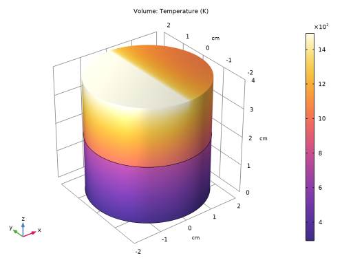
Figure 3 shows the temperature distribution in the cylinder. The composite acts as a thermal barrier resulting in a jump of the temperature over the layer.

Figure 3: Temperature distribution.

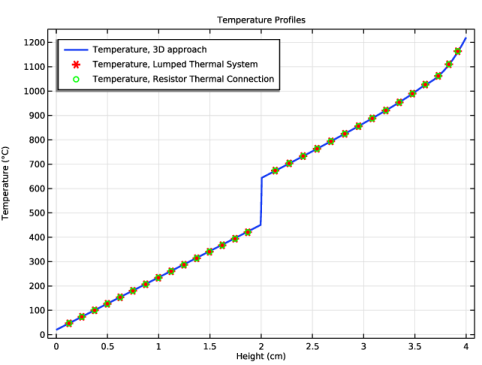
Of interest is if the lumped approach (using Heat Transfer in Shells and Lumped Thermal System) produces reliable results compared to resolving the whole steel column in 3D. This can be done with a comparative line graph as in Figure 4. Using the lumped approaches accurate results for the bulk temperatures are obtained.

Figure 4: Temperature profile for 3D and lumped approaches.

Another important question for simulating is the influence on the mesh size and on the required RAM.

With the default tetrahedral mesh of the 3D model, the number of mesh elements is about 130,000 elements and the meshing algorithm gives some warnings.

With the swept mesh feature you can significantly reduce the number of elements to about 2800 elements (prisms), which is only 2% of the initial number of elements. Note that in complex geometries the swept mesh algorithm is often not applicable.

Using the lumped approach, the number of mesh elements reduces to about 1300 elements (triangles). You can see the number of mesh elements used in the window below the window.

Notes About the COMSOL Implementation

To compare the results directly, three approaches are handled in a single MPH-file.

Heat_Transfer_Module/Tutorials,_Thin_Structure/lumped_composite_thermal_barrier_shells

Modeling Instructions

From the menu, choose .

New

In the window, click

Model Wizard

In the window, click

In the tree, select > .

Click .

Click

In the tree, select > .

Click

Global Definitions

Parameters 1

In the window, under click .

In the window for , locate the section.

In the table, enter the following settings:


Name	Expression	Value	Description
d_ceram1	50[um]	5E-5 m	Thickness of layer 1
d_ceram2	75[um]	7.5E-5 m	Thickness of layer 2
k_ceram1	1[W/(m*K)]	1 W/(m·K)	Thermal conductivity of layer 1
k_ceram2	0.5[W/(m*K)]	0.5 W/(m·K)	Thermal conductivity of layer 2
T_hot	1220[degC]	1493.2 K	Hot temperature

Geometry 1

In the window, under click .

In the window for , locate the section.

From the list, choose .

Cylinder 1 (cyl1)

In the toolbar, click

In the window for , locate the section.

In the text field, type 2.

In the text field, type 4.

In the toolbar, click

Now, create thin cylinders to define the ceramic layers between the two steel domains.

Cylinder 2 (cyl2)

In the toolbar, click

In the window for , locate the section.

In the text field, type 2.

In the text field, type d_ceram1.

Locate the section. In the text field, type 2-(d_ceram1+d_ceram2)/2.

In the toolbar, click

Cylinder 3 (cyl3)

In the toolbar, click

In the window for , locate the section.

In the text field, type 2.

In the text field, type d_ceram2.

Locate the section. In the text field, type 2-(d_ceram1+d_ceram2)/2+d_ceram1.

In the toolbar, click

Polygon 1 (pol1)

In the toolbar, click

and choose .

In the window for , locate the section.

In the table, enter the following settings:


x (cm)	y (cm)	z (cm)
0	-2	4
0	2	4

In the toolbar, click

Materials

Material Link 1 (matlnk1)

In the window, under right-click and choose > .

In the window for , locate the section.

Click

Add Material to Material Link 1 (matlnk1)

Go to the window.

In the tree, select > .

Right-click and choose .

Materials

Material Link 2 (matlnk2)

Right-click and choose > .

In the window for , locate the section.

Click

In the dialog, type 2 in the text field.

Click .

In the window for , locate the section.

Click

In the window, click .

Click

Global Definitions

Ceramic 1

In the window, under > click .

In the window for , type Ceramic 1 in the text field.

Locate the section. In the table, enter the following settings:


Property	Variable	Value	Unit	Property group
Thermal conductivity	k_iso ; kii = k_iso, kij = 0	k_ceram1	W/(m·K)	Basic
Density	rho	6000[kg/m^3]	kg/m³	Basic
Heat capacity at constant pressure	Cp	320[J/(kg*K)]	J/(kg·K)	Basic

Materials

Material Link 3 (matlnk3)

In the window, under right-click and choose > .

In the window for , locate the section.

Click

In the dialog, type 3 in the text field.

Click .

In the window for , locate the section.

Click

In the window, click .

Click

Global Definitions

Ceramic 2

In the window, under > click .

In the window for , type Ceramic 2 in the text field.

Locate the section. In the table, enter the following settings:


Property	Variable	Value	Unit	Property group
Thermal conductivity	k_iso ; kii = k_iso, kij = 0	k_ceram2	W/(m·K)	Basic
Density	rho	5800[kg/m^3]	kg/m³	Basic
Heat capacity at constant pressure	Cp	280[J/(kg*K)]	J/(kg·K)	Basic