When particles move in a high Reynolds number flow, they may interact with a large number of eddies that perturb their trajectories. The fluid velocity field used to perturb the particle trajectories is generally computed using one of the following numerical methods (Ref. 12): Reynolds-averaged Navier–Stokes (RANS), direct numerical simulation (DNS), or large eddy simulation (LES).

Although DNS (and, to some degree, LES) are capable of resolving the fluid velocity field on sufficiently small length scales so that the particle trajectories can be computed deterministically, the relatively high computational cost of these numerical methods often makes them impractical for simulation of high Reynolds number flows, particularly in complicated geometries. Instead, in the following analysis, it will be assumed that the fluid velocity field has been computed using the RANS model, in which the mean flow is simulated and variations in fluid velocity are described via the turbulent kinetic energy k (SI unit: m2/s2). When solving for the particle trajectories, the drag force is computed by first adding a random velocity perturbation to the mean flow field based on the local value of the turbulent kinetic energy.

The built-in turbulent dispersion models are dependent on the turbulent kinetic energy and on the turbulent dissipation rate ε (SI unit: m2/s3). Therefore, the accompanying fluid flow interface should use one of the following turbulence models, for which these variables are defined:

The following sections describe the available turbulent dispersion models. Each of these models can be used by selecting the appropriate option from the Turbulent Dispersion section of the settings window for the Drag Force node.

In the Continuous random walk model (Ref. 12,15,16), the evaluation of the position and velocity of a fluid element chosen at random is a Markov process. For a time step dt (SI unit: s) taken by the time-dependent solver, the general form for the change in the ith fluid velocity component dui is

where ai and bij are coefficients yet to be specified, x and u are the position and velocity of the fluid element, and dξj are the increments of a vector-valued Weiner process with independent components, which are uncorrelated Gaussian random numbers with zero mean and variance dt (Ref. 15). A more in-depth discussion of the relevance of Weiner processes in turbulent dispersion is given in Ref. 17.

In homogeneous turbulence, the velocity perturbations dui are computed by solving a classical Langevin equation (Refs. 15 and 16):

where s (SI unit: m/s) is the fluctuating rms of the velocity perturbation in any direction. For isotropic turbulence computed using the k-ε model,

In general, the Lagrangian integral time scale τL (SI unit: s) is given by (Ref. 12)

Essentially, the Lagrangian time scale characterizes the time interval size over which successively sampled random numbers should become uncorrelated. Typically τL is estimated using the functional form

where the dimensionless coefficient CL is on the order of unity. Typical values of CL have been reported in the interval [0.2,0.96] (Ref. 12) and as low as 1/7 (Ref. 16).

For isotropic turbulence, the following expression for the velocity perturbation, including the drift term, is given (Ref. 16):

The particle Stokes number St (dimensionless) is defined as

where the particle relaxation time scale τp (SI unit: s) or particle velocity response time depends on the drag law being used (see The Stokes Drag Law section) and on rarefaction effects applied to the drag force, if any (see the Drag Force in a Rarefied Flow section).

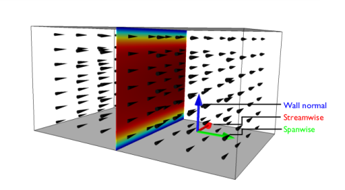
If the Continuous random walk model is used and the Include anisotropic turbulence in boundary layers check box is selected, the velocity perturbations are computed using different expressions in the streamwise, spanwise, and wall normal directions at the position of each particle.

In the following, the subscripts 1, 2, and 3 refer to the streamwise, wall normal, and spanwise directions, respectively. The streamwise direction is parallel to the fluid velocity. The wall normal direction points away from the nearest surface with a Wall boundary condition. Boundaries with the Inlet, Outlet, and Symmetry boundary conditions are not considered walls for the purpose of computing the wall normal direction. The spanwise direction is orthogonal to the streamwise and wall normal directions. Thus the streamwise, wall normal, and spanwise directions form an orthonormal basis,

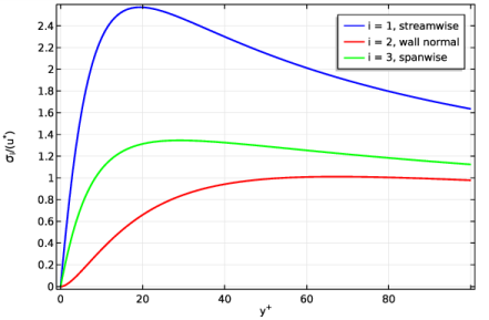
The anisotropic turbulence model differs from the isotropic Continuous random walk model when the particles are sufficiently close to walls such that y+ < 100, where y+ is the wall distance in dimensionless units,

x2 (SI unit: m) is the distance to the nearest wall, ν (SI unit: m2/s) is the fluid kinematic viscosity, and u∗ (SI unit: m/s) is the friction velocity at the nearest wall. Usually u∗ is computed by one of the turbulent flow physics interfaces.

where the rms velocity perturbations (Ref. 16) are

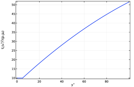
The Lagrangian time scale τL (SI unit: s) is a piecewise function of the wall distance,

The dimensionless velocity perturbations are plotted in the anisotropic region in Figure 5-4. The Lagrangian time scale is plotted in Figure 5-5.

In all other respects, the effect of these velocity perturbation terms on the particle trajectories is the same as for the isotropic Continuous random walk model.

In the Discrete random walk model (Refs. 12, 20, and 21), the components of the velocity perturbation are given instantaneous values

where ζ (dimensionless) is a vector of uncorrelated Gaussian random numbers with unit variance (Ref. 21).

Ostensibly, the velocity perturbation used in the discrete random walk model resembles the random force contributed by the Brownian Force,

However, there is a key difference in the random number sampling used to model the molecular diffusion of the Brownian Force, as opposed to the background velocity perturbation used to account for turbulent dispersion. The expression for the Brownian force includes explicit inverse-square-root dependence on the size of the time step taken by the solver. Thus, it is possible to model Brownian motion using arbitrarily small time steps and resampling the vector ζ at each step, since the reduction in the denominator compensates for the fact that the random force has less time to act on the particle and resulting in statistical convergence of the particle diffusion rate.

However, the expression for the velocity perturbation used in the discrete random walk model for turbulent dispersion has no such dependence on the time step size. If ζ is naively sampled at each time step, then as the time step size is made arbitrarily small, the effect of the turbulent kinetic energy on the particle motion will eventually become negligibly small.

To ensure that the amount of turbulent diffusion is physically meaningful, it is important that the random vector ζ is only uniquely seeded at discrete time intervals. The length of the time interval is equal to the finite (not infinitesimally small) duration of time that the particle would spend, on average, interacting with a single eddy in the flow.

In the eddy interaction model of Gosman and Ioannides (Ref. 18), the time for which the random unit vector remains in a fixed direction, here called the eddy interaction time and denoted τi, is taken as the lesser of two different time scales,

The eddy lifetime τe (SI unit: s) is the approximate duration of time between the formation and destruction of individual eddies in the flow,

where CL is a dimensionless constant.

The eddy crossing time τc (SI unit: s) is the approximate time it takes for a particle’s inertia to carry it across an eddy.

where τp is again the particle velocity response time, originally introduced in Equation 5-2 for the drag force. For Stokes drag, recall that

The dissipation length scale le (SI unit: m) is

when the physical interpretation is that the particle does not have sufficient inertia to escape from the eddy. It will instead continue to interact with the same eddy until the eddy dissipates, and hence τi = τe.

In order to define a random number seed that only changes at time intervals greater than the eddy interaction time τi, the Discrete random walk model defines an auxiliary dependent variable N (dimensionless) for the number of eddies encountered by a particle in the flow. The variable N is solved computed along the particle’s trajectory by integrating the first-order equation

The expression floor(N) is then used instead of the instantaneous time t as an argument in the random number seed used to compute the Gaussian random numbers ζi. An expression such as randomnormal(floor(N)) only takes on a new value for each integer value that N exceeds.