Radiation Pattern

•

For the RF Module and the Wave Optics Module, the variables are the far-field norm, normEfar and normdBEfar; the components of the far-field variable Efar; and the axial ratio, axialRatio and axialRatiodB.

The variables are plotted for a selected number of angles on a circle (in 2D) or a sphere (in 3D). The angle interval and the number of angles can be manually specified. Also the circle origin and radius of the circle (2D) or sphere (3D) can be specified. For 3D Radiation Pattern plots, you also specify an expression for the surface color. For 1D Radiation Pattern plots, you can optionally compute the beamwidth.

The radiation pattern plot plots a surface shape by deforming the specified circle or sphere in 2D and 3D or a circular slice in 1D. For each evaluation point on the specified circle or sphere, the plot deforms the specified circle or sphere from the evaluation point in the radial direction so that the deformed surface shape distance from the origin becomes equal to the value of the specified expression on the evaluation point on the specified circle or sphere.

The main advantage with the Radiation Pattern plot, as compared to making a Line Graph, is that the circle or sphere used for defining the plot directions is not part of the geometry for the solution. Thus, the number of plotting directions is decoupled from the discretization of the solution domain.

Radiation Pattern plots always use the spatial frame when evaluating outside the meshed domain.

To add this plot type, right-click a plot group node and choose from the menu. For nodes, you can right-click to add Deformation (2D and 3D only), Export Expressions, Graph Marker (1D only), Material Appearance, Translation, and Transparency (3D only) subnodes if desired.

	Go to Common Results Node Settings for links to information about these sections: Data, Title, Range, Inherit Style, and Coloring and Style. For 3D plot groups, see the list for Color. For Radiation Pattern plots, only Solution datasets are available as inputs.

For the standard settings, see Expressions and Predefined Quantities. In 3D, you can also select the check box and then enter a threshold value as a scalar number in the associated text field. The threshold value corresponds to the evaluated radius that maps to the plotted radius 0. The default, if the check box is cleared, is the minimum radius among those evaluated for. Additionally, in 3D, select the check box to use the radiation pattern plot expression defined in this section also as the color expression. The section is then not available.

Under , enter the . The default is 50.

Select a : (the default) or . If is selected, enter values (SI unit: deg) for

(the default is 0 degrees) and

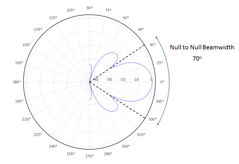
(the default is 360 degrees). If you want to compute the beamwidth, select from the list. Then, a field appears, where you can specify a nonnegative number to compute the beamwidth at a certain level down from the reference direction. The unit for that level is the same as the unit for the expression used in the radiation pattern plot (dB, for example, for an exterior-field sound pressure level). The beamwidth is the width of the lobe around the reference direction (in degrees). When you compute the beamwidth, the computed values appear in a table with columns for the parameter (typically a frequency), the beamwidth, and the null-to-null beamwidth (the angular separation from which the magnitude of the radiation pattern decreases to zero away from the main beam; see the figure below).

Note that the beamwidth calculation only makes sense if there is a main lobe in the reference direction.

For 1D Radiation Pattern plot nodes referring to a solution in a 2D axisymmetric or 3D component, under enter the coordinate at the center of the evaluation circle. Under specify the normal to the circular slice of the far-field bulb. The default normal is {0, 0, 1} for the normal using 3D components and {0, 1, 0} for the normal using 2D axisymmetric components.

If a Pressure Acoustics interface is used in the component from which the dataset is taken, you can also add a (SI unit: m) under for a radius-dependent exterior-field expression.

Under specify a reference direction from which the angle is measured. The entered vector is projected onto the evaluation plane. The default direction is {1, 0, 0} for the reference direction using 3D components, {0, 0, 1} for 2D axisymmetric components, and {1, 0} for 2D components.

A schematic of the evaluation circle is depicted in Figure 21-6. In 3D, you can preview the evaluation circle in the geometry by clicking the button at the bottom of the section. An example of the resulting plot is depicted in Figure 21-7.

Under , enter the . The default is 10. Enter the . The default is 20.

Select a : (the default) or . If is selected in a 3D plot group, you can also select or from the list. If the list is set to , you can enter or select an expression for the directivity in the field. The direction for the strongest radiation and the directivity value (also in dB) display in a table window (see The Table Window and Tables Node). So if, for example, you model a speaker that is located in an infinite baffle (and symmetry is used in the radiation pattern calculation), then plot and evaluate the whole field to get the directivity.

If is selected, enter values (SI unit: deg) for:

If a pressure acoustics interface is used in the component from which the dataset is taken, you can also specify the following settings for a radius-dependent exterior-field expression. Under from the list, select (the default) or . If is selected, enter values for the , , and coordinates at the center of the sphere (SI unit: m). The default is 0. Enter a (SI unit: m). The default is 1 m.

For 2D axisymmetric radiation pattern plots, you can evaluate the azimuthal (

) angle once for each angle when you specify a name of the variable for the (

) angle in the field and use it in the expression for the radiation pattern. Doing so slows down the evaluation, so if the field is empty, an evaluate-once-and-revolve approach is used instead.

This section is available in 1D plot groups only. Select the check box to display the plotted expressions to the right of the plot. In plots where each line represents a certain time value, eigenvalue, or parameter value, these values are also displayed.

When is selected from the list (the default), the legend texts appear automatically. You can add a prefix or a suffix to the automatic legend text in the and fields. If is selected from the list, enter your own legend text into the table. If is selected, you can use the eval function to create an evaluated legend text in the field that include evaluated global expressions such as global parameters used in sweeps. For the numerical evaluation, you can control the precision in the field (default: 3).