Directivity
The Directivity plot () is an extension of the far-field plots and is a common acoustic plot for speakers, for example. The plot collects spatial information across frequencies and shows this information in a contour plot.
You can add Directivity plot nodes to 1D and 2D plot groups from the More Plots submenu.
Go to Common Results Node Settings for links to information about these sections: Data, Title, Levels, Range, Inherit Style, and Coloring and Style. See below for some specific settings in the Coloring and Style section.
Expression
For the standard settings, see Expressions and Predefined Quantities. You can also choose a normalization of the data from the Normalization list:
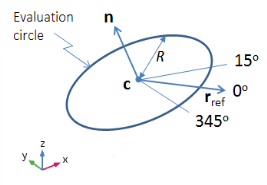
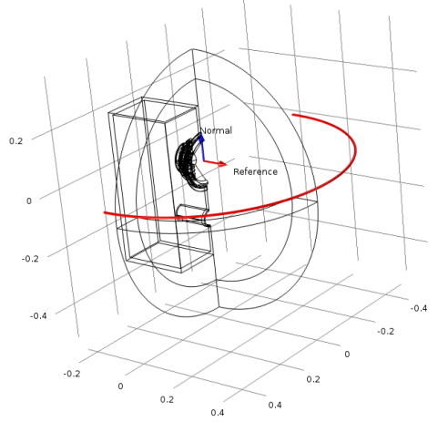
Choose With respect to angle (the default) to compute an expression with the level normalized with respect to the value at a specific angle. You specify the angle (in degrees) in the Angle field (unit: deg).
Choose With respect to maximum to compute the expression normalized with respect to its maximum level value for each frequency.
Choose None to not use any normalization.
Evaluation
Under Angles, enter the Number of angles. The default is 50.
Select a Restriction: None (the default) or Manual.
If Manual is selected, enter values (SI unit: deg) for:
start (the default is 0 degrees).
range (the default is 360 degrees). Typically the range will be 180 degrees to evaluate the directivity in the half space in front of a speaker.
The following settings only appear if there is a physics interface in the model that makes use of them. Under Center, enter values for the coordinates at the center of the evaluation circle. Under Normal vector, enter the components of the normal vector defining the evaluation plane in the x, y, and z fields. Under Evaluation distance (only available when applicable), enter a Radius for the evaluation; the default is 1 m as usually used for these plots. Under Reference direction, specify the coordinates of the vector that specifics the direction representing 0 degrees in the plot. The entered vector is projected onto the evaluation plane. A schematic of the evaluation circle is given in Figure 21-6 below.
Figure 21-6: Schematic of the evaluation circle used in the Directivity and Radiation Pattern plots, showing the circle center c, evaluation plane normal n, evaluation radius R, and reference direction rref.
In 3D and 2D axisymmetric models, you can preview the evaluation plane, including circle, normal, and reference direction, in the geometry by clicking the Preview Evaluation Plane button at the bottom of the Evaluation section. An example of the resulting plot is depicted in Figure 21-7 below.
Figure 21-7: Preview plot of the evaluation circle used in the directivity plot for the Vented Loudspeaker Enclosure model from the Acoustics Module Application Gallery.
Coloring and Style
In addition to common coloring and style settings, you can specify the axis and scale for the frequency and the contour type.
From the Layout list, choose:
Frequency on x-axis to plot with the frequency on the x-axis.
Frequency on y-axis to plot with the frequency on the y-axis.
From the Frequency scale list (2D only), choose:
Logarithmic (the default) to plot the frequency using a logarithmic scale.
Linear to plot the frequency using a linear scale.
Select a Contour type: Line or Filled (the default). Using filled contours creates a plot with color banding rather than isolated contour lines.
If Line is selected, you can also select the Level labels check box to display line labels on the graph. When that check box is selected, you can specify a numerical precision in the Precision field (default: 4). In 1D, you can also specify a line width in the Width field (default: Default from preferences) in 1D.
If Filled is selected, you can also clear the Fill surfaces outside of contour levels check box (selected by default) to not fill the areas of the geometry’s surface that are above the highest and below the lowest contour.