|
•
|
Layered Linear Elastic Material in the Shell interface (requires the Composite Materials Module).
|
|
•
|
Thin Layer in the Heat Transfer in Solids interface.
|
|
•
|
The most common place is under Global Definitions>Materials. When you reference a layered material from a physics interface, you do it indirectly through either a Layered Material Link or a Layered Material Link (Subnode) under Materials in the current component.
|
|
•
|
It can also be a subnode under a Layered Material Stack node in a component.
|
|
•
|
Click the Blank Material (
|
|
•
|
Click the Add Material from Library (
|
|
•
|
Click the Go to Material (
|
|
|
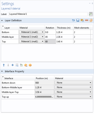
When loading a file, the second column containing the material tag is ignored. The reason is that there is no way to ascertain that a material tag like ‘mat2’ would point to the same material in another context. You can even load a file where that column is absent.
|
|
•
|
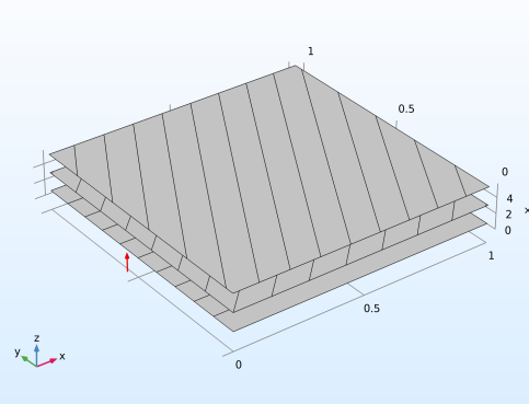
In a layer stack preview plot, it controls the height of the stack in the z direction. For laminates with many layers, you may need to increase this value.
|
|
•
|
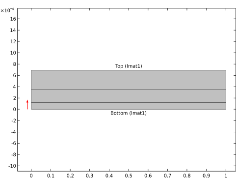
In the layer cross section preview plot, it controls the height in the y direction. The width is always unity.
|