PDF

Uncertainty Quantification of the Ishigami Function
Introduction
This example demonstrates how to perform uncertainty quantification analysis of the Ishigami function. This random function of three variables is a well-known benchmark used to test global sensitivity analysis and uncertainty quantification algorithms. The mean, standard deviation, maximum, and mininum values as well as Sobol indices of the Ishigami function can be calculated analytically for the input distributions used here.
For this test problem, the Ishigami function is
where X1, X2, and X3 are independent uniformly distributed random variables in [−π,+π] with a = 7 and b = 0.1.
The function can be visualized in 3D by using, for example, a slice plot as in Figure 1.
Figure 1: Slice plot of the Ishigami function.
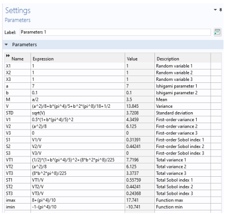
The analytically computed values are according to Table 1.
For reference, these values are entered as global parameters in the model.
Model Definition
The model runs through 3 uncertainty quantification studies: Screening, Sensitivity analysis, and Uncertainty Propagation using the Ishigami function as the quantity of interest. In order to perform the uncertainty quantification analysis, the three random variables need to be defined as global parameters using arbitrary values. The actual values for these variables will, during the simulation, be randomized by the uncertainty quantification algorithms. All the global parameters in the model are shown in Figure 2.
Figure 2: The model parameters.
The Ishigami function is defined as an analytic function with three input arguments as shown in Figure 3.
Figure 3: The Ishigami function entered as an Analytic function, ishigami.
Results and Discussion
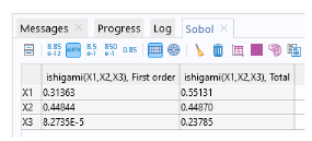
The sensitivity analysis shows that the computed Sobol indices are consistent with the true analytical values, as shown in Figure 4 below.
Figure 4: The computed Sobol indices.
Similarly, the values for mean, standard deviation (STD), minimum, and maximum are consistent with the analytical values, as shown in Figure 5.
Figure 5: The computed values for mean, standard deviation, minimum, maximum, and confidence intervals.
The accuracy of the results can be increased by lowering tolerances or increasing the number of sample input points.
The computed kernel density estimation is displayed in Figure 6.
Figure 6: The KDE plot for the Ishigami function.
These uncertainty quantification results can be compared not only with the analytical values but also with that of the direct Monte Carlo simulation performed in the model Direct Monte Carlo Simulation of the Ishigami Function.
Reference
1. T. Ishigami and T. Homma, “An importance quantification technique in uncertainty analysis for computer models,” Proc. First Int’l Symp. Uncertainty Modeling and Analysis, IEEE, pp. 398-403, 1990.
Application Library path: Uncertainty_Quantification_Module/Tutorials/ishigami_function_uncertainty_quantification
Modeling Instructions
From the File menu, choose New.
New
In the New window, click  Blank Model.
Add Study
1
In the Home toolbar, click  Add Study to open the Add Study window.
2
Go to the Add Study window.
3
Find the Studies subsection. In the Select Study tree, select Preset Studies for Selected Physics Interfaces>Stationary.
4
Click Add Study in the window toolbar.
5
In the Home toolbar, click  Add Study to close the Add Study window.
Global Definitions
Parameters 1
1
In the Model Builder window, under Global Definitions click Parameters 1.
2
In the Settings window for Parameters, locate the Parameters section.
3
Ishigami Function
1
In the Home toolbar, click  Functions and choose Global>Analytic.
2
In the Settings window for Analytic, type ishigami in the Function name text field.
3
Locate the Definition section. In the Expression text field, type sin(x1)+a*(sin(x2))^2+b*x3^4*sin(x1).
4
In the Arguments text field, type x1,x2,x3.
5
In the Label text field, type Ishigami Function.
6
Locate the Plot Parameters section. In the table, enter the following settings:
7
Click  Create Plot.
Results
3D Plot Group 1
Study 1
Uncertainty Quantification
1
In the Model Builder window, right-click Study 1 and choose Uncertainty Quantification>Uncertainty Quantification.
2
In the Settings window for Uncertainty Quantification, locate the Quantities of Interest section.
3
4
5
Locate the Input Parameters section. Find the Input parameters table subsection. Click  Add three times.
6
7
In the Home toolbar, click  Compute.
Results
MOAT, ishigami(X1,X2,X3)
The Screening study shows that all parameters are influential and that the parameter X3 has a nonlinear influence on the Ishigami function, or that it is interacting with the other input parameters, or both.
Study 1
Uncertainty Quantification
In the Model Builder window, under Study 1 right-click Uncertainty Quantification and choose Add New Uncertainty Quantification Study For>Sensitivity Analysis.
Study 2
Uncertainty Quantification
To achive a high level of accuracy, change from the default Compute type, which is Improve and analyze, to Compute and analyze. This option will not reuse any results from previous model evaluations but instead start from scratch.
1
In the Model Builder window, under Study 2 click Uncertainty Quantification.
2
In the Settings window for Uncertainty Quantification, locate the Uncertainty Quantification Settings section.
3
From the Compute action list, choose Compute and analyze.
4
In the Home toolbar, click  Compute.
The Sensitivity analysis study computes Sobol indices that are consistent with the analytical values.
5
Right-click Study 2>Uncertainty Quantification and choose Add New Uncertainty Quantification Study For>Uncertainty Propagation.
Study 3
Uncertainty Quantification
Now, change the Surrogate model to Adaptive sparse polynomial chaos expansion. For the Ishigami function, the polynomical chaos expansion surrogate model turns out to be much more efficient than the default Adaptive Gaussian process option.
1
In the Model Builder window, under Study 3 click Uncertainty Quantification.
2
In the Settings window for Uncertainty Quantification, locate the Uncertainty Quantification Settings section.
3
Find the Surrogate model settings subsection. From the Surrogate model list, choose Adaptive sparse polynomial chaos expansion.
Again, to achive a high level of accuracy, change to Compute and analyze. This option will not reuse any results from previous model evaluations but instead start from scratch.
4
From the Compute action list, choose Compute and analyze.
5
In the Home toolbar, click  Compute.