PDF

Direct Monte Carlo Simulation of the Ishigami Function
Introduction
This example demonstrates how to perform a direct Monte Carlo simulation of the Ishigami function. This random function of three variables is a well-known benchmark used to test global sensitivity analysis and uncertainty quantification algorithms. The mean, standard deviation, maximum, and mininum values of the Ishigami function can be calculated analytically for the input distributions used here.
For this test problem, the Ishigami function is
where X1, X2, and X3 are independent uniformly distributed random variables in [−π,+π] with a = 7 and b = 0.1.
The analytically computed values are according to Table 1.
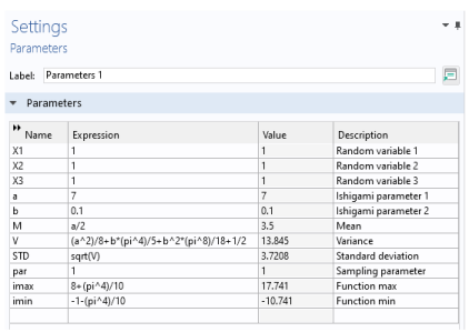
For reference, these values are entered as global parameters in the model.
Model Definition
In order to perform a direct Monte Carlo simulation, the three random variables need to be defined as global parameters using arbitrary values. The actual values for these variables during the simulation will be randomized. Figure 1 shows all global parameters in the model.
Figure 1: The model parameters.
The Sampling parameter par is used to generate vector of random values for the random variables X1, X2, and X3.
The Ishigami function is defined as an analytic function with three input arguments.
Figure 2: The Ishigami function entered as an Analytic function, ishigami.
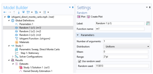
Three uniform random functions — rn1, rn2, and rn2 — are defined and later used in the Monte Carlo simulation. Each of the random variables has a unique random seed to ensure that they emulate independent random variables.
Figure 3: The random functions used for the Monte Carlo simulation.
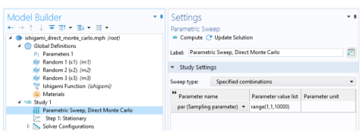
The main part of the simulation is a Parametric Sweep and a Stationary study. The Stationary study is necessary to generate all function values used for the results processing. In the model, 10,000 sample points are generated for each of the random variables. This is achieved by running a parametric sweep between 1 and 10,000 in steps of 1. To increase the accuracy of the simulation you can easily increase this value by 10 or 100 times.
Figure 4: The Parametric Sweep definition used for the Monte Carlo simulation.
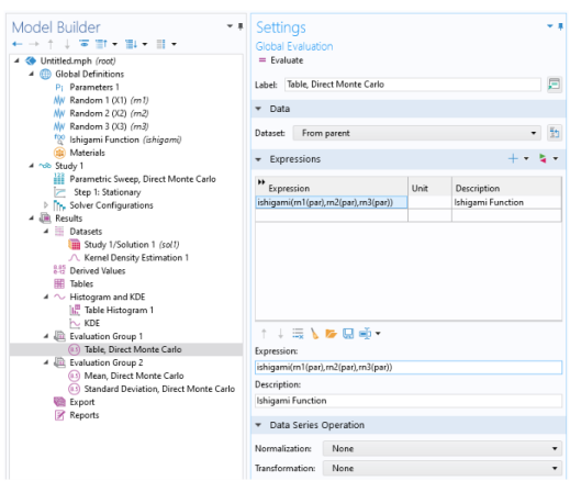
The Monte Carlo simulation is performed by means of an Evaluation Group that outputs the simulated function values to a table.
Figure 5: The Evaluation Group used to evaluate the Ishigami function.
Results and Discussion
The results compares a Table Histogram plot with a KDE plot (kernel density estimation).
Figure 6: A Table Histogram plot and KDE plot.
The mean and standard deviation are computed as Data Series Operations on the Evaluation Group table.
Figure 7: The computed mean and standard deviation.
These values should be compared with the analytical values of the mean and standard deviation of 3.5 and 3.7208, respectively. To get higher accuracy, increase the number of steps in the sweep.
Reference
1. T. Ishigami and T. Homma, “An importance quantification technique in uncertainty analysis for computer models,” Proc. First Int’l Symp. Uncertainty Modeling and Analysis, IEEE, pp. 398-403, 1990.
Application Library path: Uncertainty_Quantification_Module/Tutorials/ishigami_function_direct_monte_carlo
Modeling Instructions
From the File menu, choose New.
New
In the New window, click  Blank Model.
Add Study
1
In the Home toolbar, click  Add Study to open the Add Study window.
2
Go to the Add Study window.
3
Find the Studies subsection. In the Select Study tree, select Preset Studies for Selected Physics Interfaces>Stationary.
4
Click Add Study in the window toolbar.
5
In the Home toolbar, click  Add Study to close the Add Study window.
Global Definitions
Parameters 1
1
In the Model Builder window, under Global Definitions click Parameters 1.
2
In the Settings window for Parameters, locate the Parameters section.
3
Random 1 (X1)
1
In the Home toolbar, click  Functions and choose Global>Random.
2
In the Settings window for Random, type Random 1 (X1) in the Label text field.
3
Locate the Parameters section. In the Range text field, type 2*pi.
4
Select the Use random seed check box.
Random 2 (X2)
1
In the Home toolbar, click  Functions and choose Global>Random.
2
In the Settings window for Random, type Random 2 (X2) in the Label text field.
3
Locate the Parameters section. In the Range text field, type 2*pi.
4
Select the Use random seed check box.
Random 3 (X3)
1
In the Home toolbar, click  Functions and choose Global>Random.
2
In the Settings window for Random, type Random 3 (X3) in the Label text field.
3
Locate the Parameters section. In the Range text field, type 2*pi.
4
Select the Use random seed check box.
Ishigami Function
1
In the Home toolbar, click  Functions and choose Global>Analytic.
2
In the Settings window for Analytic, type ishigami in the Function name text field.
3
Locate the Definition section. In the Expression text field, type sin(x1)+a*(sin(x2))^2+b*x3^4*sin(x1).
4
In the Arguments text field, type x1,x2,x3.
5
In the Label text field, type Ishigami Function.
Study 1
Parametric Sweep, Direct Monte Carlo
1
In the Study toolbar, click  Parametric Sweep.
2
In the Settings window for Parametric Sweep, type Parametric Sweep, Direct Monte Carlo in the Label text field.
3
Locate the Study Settings section. Click  Add.
4
5
In the Study toolbar, click  Compute.
Results
Evaluation Group 1
1
In the Model Builder window, expand the Results node.
2
Right-click Results and choose Evaluation Group.
Table, Direct Monte Carlo
1
In the Model Builder window, right-click Evaluation Group 1 and choose Global Evaluation.
2
In the Settings window for Global Evaluation, locate the Expressions section.
3
4
In the Evaluation Group 1 toolbar, click  Evaluate.
5
In the Label text field, type Table, Direct Monte Carlo.
Evaluation Group 2
In the Results toolbar, click  Evaluation Group.
Mean, Direct Monte Carlo
1
Right-click Evaluation Group 2 and choose Global Evaluation.
2
In the Settings window for Global Evaluation, type Mean, Direct Monte Carlo in the Label text field.
3
Locate the Expressions section. In the table, enter the following settings:
4
Locate the Data Series Operation section. From the Transformation list, choose Average.
Standard Deviation, Direct Monte Carlo
1
In the Model Builder window, right-click Evaluation Group 2 and choose Global Evaluation.
2
In the Settings window for Global Evaluation, type Standard Deviation, Direct Monte Carlo in the Label text field.
3
Locate the Expressions section. In the table, enter the following settings:
4
Locate the Data Series Operation section. From the Transformation list, choose Standard deviation.
Evaluation Group 2
1
In the Model Builder window, click Evaluation Group 2.
2
In the Evaluation Group 2 toolbar, click  Evaluate.
Kernel Density Estimation 1
1
In the Model Builder window, expand the Results>Datasets node.
2
Right-click Results>Datasets and choose More Datasets>Kernel Density Estimation.
3
In the Settings window for Kernel Density Estimation, locate the Data section.
4
From the Source list, choose Evaluation group.
5
Find the Columns subsection. From the x-coordinates list, choose Ishigami Function.
6
Click to expand the Advanced section.
Histogram and KDE
1
In the Results toolbar, click  1D Plot Group.
2
In the Settings window for 1D Plot Group, type Histogram and KDE in the Label text field.
Table Histogram 1
1
In the Histogram and KDE toolbar, click  More Plots and choose Table Histogram.
2
In the Settings window for Table Histogram, locate the Data section.
3
From the Source list, choose Evaluation group.
4
From the x-coordinates list, choose Ishigami Function.
5
Locate the Bins section. In the Number text field, type 200.
6
Locate the Output section. From the Normalization list, choose Integral.
7
Click to expand the Coloring and Style section.
KDE
1
In the Model Builder window, right-click Histogram and KDE and choose Line Graph.
2
In the Settings window for Line Graph, type KDE in the Label text field.
3
Locate the y-Axis Data section. In the Expression text field, type kde1val.
4
Locate the Data section. From the Dataset list, choose Kernel Density Estimation 1.
5
In the Histogram and KDE toolbar, click  Plot.
6
Click the  Zoom Extents button in the Graphics toolbar.