PDF

Various Analyses of an Elbow Bracket
Introduction
The component shown in Figure 1 is part of a support mechanism and is subjected to various loads. This tutorial model takes you through the steps to carry out a detailed analysis of the part using the Structural Mechanics Module.
Figure 1: Geometry of the elbow bracket.
In the various parts of the example you are introduced to using some basic analysis types, together with numerous postprocessing possibilities. These analysis types are:
This tutorial model comes in two versions:
A short version, elbow_bracket_brief, treating the three first analysis types in the above list.
A complete version, elbow_bracket, treating all nine analysis types.
This tutorial model consists of a single model, with nine studies, corresponding to these analysis types, which are described in the section Study Types in the Structural Mechanics Module User’s Guide. The chapter Structural Mechanics Modeling in the same manual provides further assistance.
Note: If you have already built the short model version described in the section Static and Eigenfrequency Analyses of an Elbow Bracket, you can proceed directly to the section Time-Dependent Analysis.
Model Definition
The geometry for this part, see Figure 1, has been created with a CAD software, and it is available for you to import into COMSOL Multiphysics.
Material
The material is structural steel, as taken from the material library, with Young’s modulus 200 GPa and Poisson’s ratio of 0.33.
Damping
The Structural Mechanics Module supports several types damping for dynamic analysis. You can also use no damping, which is the default option.
In some of the studies Rayleigh damping is used. It is defined by two scalar damping parameters that are multipliers to the mass matrix (αdM) and stiffness matrix (βdK) in the following way:
where C is the damping matrix, M is the mass matrix, and K is the stiffness matrix. The damping is specified locally in each domain; this means that you can specify different damping parameters in different parts of the model. This is an extension of the common definition of Rayleigh damping.
To find values for the Rayleigh damping parameters, you can use the relations between the critical damping ratio and the Rayleigh damping parameters. It is often easier to interpret the critical damping ratios, which are given by
where ξi is the critical damping ratio at a specific angular frequency ωi. Knowing two pairs of corresponding ξi and ωi results in a system of equations from which the damping parameters can be determined. This method of determining the Rayleigh damping parameters is built-in.
Assume that the structure has a constant damping ratio of 0.1. Select two frequencies near the excitation frequency, 400 Hz and 600 Hz. This will result in αdM = 302 s-1 and βdK = 3.18·105 s.
For more information see the section Mechanical Damping and Losses in the Structural Mechanics Module User’s Guide.
If modal based dynamic response studies are performed it is usually easier to give the critical damping ratios directly. This also gives more detailed control over the damping properties over a large frequency range.
Loads and Constraints
The displacement are fixed in all directions on the face shown in Figure 2. The load is described under each study, but in all cases it is distributed over the face as shown in this figure.
Figure 2: Constraint and loading of the bracket.
The Application Libraries note immediately below appears in the discussion of every model. The path indicates the location of the example file in the Application Libraries root directory. The most convenient way to open it is from the Application Libraries window in the COMSOL Desktop, which you can open from the File menu.
Application Library path: Structural_Mechanics_Module/Tutorials/elbow_bracket
Modeling Instructions
From the File menu, choose New.
New
In the New window, click  Model Wizard.
Model Wizard
1
In the Model Wizard window, click  3D.
2
In the Select Physics tree, select Structural Mechanics>Solid Mechanics (solid).
3
Click Add.
4
Click  Study.
5
In the Select Study tree, select General Studies>Stationary.
6
Geometry 1
Import 1 (imp1)
1
In the Home toolbar, click  Import.
2
In the Settings window for Import, locate the Import section.
3
From the Source list, choose COMSOL Multiphysics file.
4
Click  Browse.
5
6
Click  Import.
7
Click the  Wireframe Rendering button in the Graphics toolbar.
The view in the Graphics window should look like that in the image below.
8
Click the  Wireframe Rendering button in the Graphics toolbar to return to the default surface rendering.
Suppress some edges during meshing, in order to avoid generation of unnecessary small elements.
Ignore Edges 1 (ige1)
1
In the Geometry toolbar, click  Virtual Operations and choose Ignore Edges.
2
On the object fin, select Edges 17, 21, 23, 27, 38, 40, 42, and 44 only.
It might be easier to select the correct edges by using the Selection List window. To open this window, in the Home toolbar click Windows and choose Selection List. (If you are running the cross-platform desktop, you find Windows in the main menu.)
Mesh 1
Free Tetrahedral 1
In the Mesh toolbar, click  Free Tetrahedral.
Size
There are nine predefined combinations of mesh parameter settings. They range from Extremely fine to Extremely coarse, with Normal as the default setting. Unless any other mesh parameters are set, this is the setting that is used if you use Build All or Build Selected to generate the mesh.
As a stress concentration can be expected in the corner of the bracket, put a finer mesh there.
Size 1
1
In the Model Builder window, right-click Free Tetrahedral 1 and choose Size.
2
In the Settings window for Size, locate the Geometric Entity Selection section.
3
From the Geometric entity level list, choose Boundary.
4
Locate the Element Size section. From the Predefined list, choose Extra fine.
5
6
In the Model Builder window, right-click Mesh 1 and choose Build All.
Materials
Next, specify the material properties. You can do this either by explicitly typing them in or by selecting a library material in the Material Browser. For this model, use a library material.
Add Material
1
In the Home toolbar, click  Add Material to open the Add Material window.
2
Go to the Add Material window.
3
In the tree, select Built-in>Structural steel.
4
Click Add to Component in the window toolbar.
In the Home toolbar, click  Add Material to close the Add Material window.
Static Analysis
A static analysis has no explicit or implicit time dependencies. This situation corresponds to the steady state with constant (in time) boundary conditions and material properties.
The purpose of such analysis can be to find the maximum stress level and compare it with the material’s yield strength, as well as to check that the deformation of the component is within the limits of the design criteria.
Results and Discussion
The analysis shows that the von Mises equivalent stress has a maximum value of about190 MPa, which, compared with the material’s yield strength of 350 MPa, results in a utilization factor of 54%.
The analysis also gives the maximum static displacements as 1.14 mm
Three different representations of the stress state are shown in Figure 3 through Figure 5.
Figure 3: Equivalent stresses on the boundary of the domain.
Figure 4: Isosurface plot of the equivalent stress.
Figure 5: Arrow plot of the principal stresses.
Modeling Instructions
Solid Mechanics (solid)
Fixed Constraint 1
1
In the Model Builder window, under Component 1 (comp1) right-click Solid Mechanics (solid) and choose Fixed Constraint.
2
Boundary Load 1
1
In the Physics toolbar, click  Boundaries and choose Boundary Load.
2
3
In the Settings window for Boundary Load, locate the Force section.
4
Specify the FA vector as
Study 1 (Static)
In this model, where there are many different studies, it is a good idea to assign manual names to some nodes in the model tree.
1
In the Model Builder window, click Study 1.
2
In the Settings window for Study, type Study 1 (Static) in the Label text field.
The default settings in the generated solver are OK for this model, so it can be run directly.
3
In the Home toolbar, click  Compute.
Before moving on to analyzing the solution, rename the solver.
Solution, Static
1
In the Model Builder window, expand the Study 1 (Static)>Solver Configurations node, then click Solution 1 (sol1).
2
In the Settings window for Solution, type Solution, Static in the Label text field.
Results
Similarly, rename the solution dataset.
Static Solution
1
In the Model Builder window, expand the Results>Datasets node, then click Study 1 (Static)/Solution, Static (sol1).
2
In the Settings window for Solution, type Static Solution in the Label text field.
In the Results branch, you can create various plot types, evaluate expressions, or animate the results. The result features can visualize any expression containing, for example, the solution variables, their derivatives, and the space coordinates. Many frequently used expressions are predefined as postprocessing variables, and they are directly available in the Expression section menus for the various plot types.
When the solver finishes, a default plot appears. It shows a volume plot of the von Mises stress with the deformed shape of the component. For future reference, you can rename it.
Static Stress Contour
1
In the Model Builder window, under Results click Stress (solid).
2
In the Settings window for 3D Plot Group, type Static Stress Contour in the Label text field.
Volume 1
1
In the Model Builder window, expand the Static Stress Contour node, then click Volume 1.
2
In the Settings window for Volume, locate the Expression section.
3
From the Unit list, choose MPa.
4
In the Static Stress Contour toolbar, click  Plot.
5
Click the  Zoom Extents button in the Graphics toolbar.
The applied loads are also available in a default plot.
Applied Loads, Static Solution
1
In the Model Builder window, under Results click Applied Loads (solid).
2
In the Settings window for Group, type Applied Loads, Static Solution in the Label text field.
Boundary Loads (solid)
In the Model Builder window, expand the Applied Loads, Static Solution node.
In order not to hide any load vectors, a wireframe representation is used for the geometry as a default. The plot group is however prepared for a visualization with hidden surfaces.
Gray Surfaces
In the Model Builder window, expand the Boundary Loads (solid) node.
Transparency 1
1
In the Model Builder window, expand the Gray Surfaces node.
2
Right-click Transparency 1 and choose Disable.
Boundary Loads (solid)
1
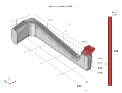
In the Model Builder window, under Results>Applied Loads, Static Solution click Boundary Loads (solid).
2
In the Boundary Loads (solid) toolbar, click  Plot.
To evaluate the maximum displacement, use a nonlocal maximum coupling.
Definitions
Maximum 1 (maxop1)
1
In the Definitions toolbar, click  Nonlocal Couplings and choose Maximum.
2
In the Settings window for Maximum, locate the Source Selection section.
3
From the Geometric entity level list, choose Boundary.
4
From the Selection list, choose All boundaries.
Variables 1
1
In the Definitions toolbar, click  Local Variables.
2
In the Settings window for Variables, locate the Variables section.
3
Study 1 (Static)
Solution, Static (sol1)
1
In the Model Builder window, under Study 1 (Static)>Solver Configurations right-click Solution, Static (sol1) and choose Solution>Update.
This step is necessary in order to access variables that were created after the solution was performed.
Results
Global Evaluation 1
1
In the Results toolbar, click  Global Evaluation.
2
In the Settings window for Global Evaluation, click Replace Expression in the upper-right corner of the Expressions section. From the menu, choose Component 1 (comp1)>Definitions>Variables>U_max - Maximum deflection - m.
3
Locate the Expressions section. In the table, enter the following settings:
4
Click  Evaluate.
The result, approximately 1.1 mm appears in the Table window.
Next, add a second plot group and create an isosurface plot. The resulting plot should resemble that in Figure 4.
Static Stress Isosurface
1
In the Results toolbar, click  3D Plot Group.
2
In the Settings window for 3D Plot Group, type Static Stress Isosurface in the Label text field.
Isosurface 1
1
Right-click Static Stress Isosurface and choose Isosurface.
2
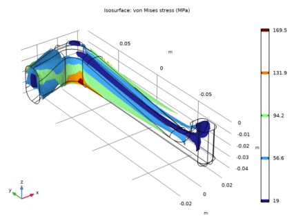
In the Settings window for Isosurface, click Replace Expression in the upper-right corner of the Expression section. From the menu, choose Component 1 (comp1)>Solid Mechanics>Stress>solid.mises - von Mises stress - N/m².
3
Locate the Expression section. From the Unit list, choose MPa.
Deformation 1
1
Right-click Isosurface 1 and choose Deformation.
2
Click the  Go to Default View button in the Graphics toolbar.
With the following steps you can reproduce the principal stress arrow plot shown in Figure 5:
Static Principal Stress Arrow Plot
1
In the Results toolbar, click  3D Plot Group.
2
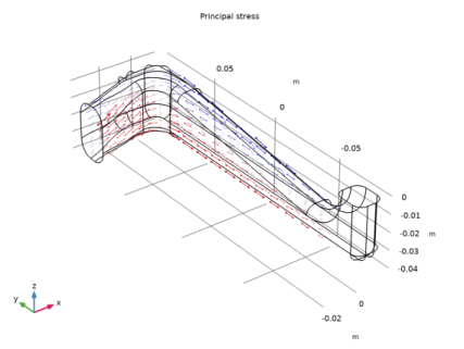
In the Settings window for 3D Plot Group, type Static Principal Stress Arrow Plot in the Label text field.
Principal Stress Volume 1
1
In the Static Principal Stress Arrow Plot toolbar, click  More Plots and choose Principal Stress Volume.
2
In the Settings window for Principal Stress Volume, locate the Positioning section.
3
Find the X grid points subsection. In the Points text field, type 10.
4
Find the Y grid points subsection. In the Points text field, type 15.
5
Find the Z grid points subsection. In the Points text field, type 10.
In the Static Principal Stress Arrow Plot toolbar, click  Plot.
Eigenfrequency Analysis
An eigenfrequency analysis finds the eigenfrequencies and modes of deformation of a component. The eigenfrequencies f in the structural mechanics field are related to the eigenvalues λ returned by the solvers through
In COMSOL Multiphysics you can choose between working with eigenfrequencies and working with eigenvalues according to your preferences. Eigenfrequencies is the default option for all physics interfaces in the Structural Mechanics Module.
If no damping is included in the material, the undamped natural frequencies are computed.
The purpose of the following eigenfrequency analysis is to find the six lowest eigenfrequencies and corresponding mode shapes.
Results and Discussion
The first six eigenfrequencies are:
f1
f2
f3
f4
f5
f6
The mode shapes corresponding to the two lowest eigenfrequencies are shown in Figure 6. The deformed plot indicates an oscillation in the xy-plane for the lowest eigenfrequency, while the second lowest eigenmode shows an oscillation in the yz-plane.
Figure 6: Eigenmodes of the two lowest eigenfrequencies.
Notes About the COMSOL Implementation
Any loads present on the model, such as the load from the static load case above, are ignored in the default eigenfrequency analysis. It is also possible to include effects from prestress. You can find an example of such an analysis in the example Vibrating String.
Modeling Instructions
Add a new study to your model.
Add Study
1
In the Home toolbar, click  Add Study to open the Add Study window.
2
Go to the Add Study window.
3
Find the Studies subsection. In the Select Study tree, select General Studies>Eigenfrequency.
4
Click Add Study in the window toolbar.
5
In the Home toolbar, click  Add Study to close the Add Study window.
Study 2 (Eigenfrequency)
1
In the Model Builder window, click Study 2.
2
In the Settings window for Study, type Study 2 (Eigenfrequency) in the Label text field.
3
In the Home toolbar, click  Compute.
Solution, Eigenfrequency
1
In the Model Builder window, expand the Study 2 (Eigenfrequency)>Solver Configurations node, then click Solution 2 (sol2).
2
In the Settings window for Solution, type Solution, Eigenfrequency in the Label text field.
Results
Eigenfrequency Solution
1
In the Model Builder window, under Results>Datasets click Study 2 (Eigenfrequency)/Solution, Eigenfrequency (sol2).
2
In the Settings window for Solution, type Eigenfrequency Solution in the Label text field.
Undamped Mode Shapes
As a default, the first eigenmode is shown. Follow these steps to reproduce the plot in the left panel of Figure 6.
Take a look at the second mode as well.
1
In the Model Builder window, under Results click Mode Shape (solid).
2
In the Settings window for 3D Plot Group, locate the Data section.
3
From the Eigenfrequency (Hz) list, choose 573.44.
4
In the Mode Shape (solid) toolbar, click  Plot.
Compare the resulting plot to that to the right in Figure 6.
You can give the plot a more descriptive name:
5
In the Label text field, type Undamped Mode Shapes.
Animation 1
In the Undamped Mode Shapes toolbar, click  Animation and choose Player.
Mode Shape Animation
This creates an animation showing how the elbow bracket would deform if subjected to a harmonic load with a frequency near the selected eigenfrequency, in this case 571 Hz. To play the movie again, click the Play button in the Graphics toolbar.
The default animation sequence type when you add a player this way is Dynamic data extension. If you set the Sequence type to Stored solutions and then click the Generate Frame button, you get an animation where each frame corresponds to an eigenmode in the Eigenfrequency list. By using the Frame number slider in the Frames section you can then easily browse the eigenmodes.
Rename the player:
1
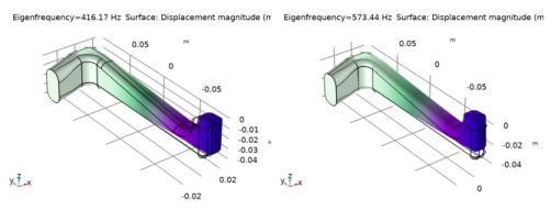
In the Model Builder window, expand the Results>Undamped Mode Shapes node, then click Results>Export>Animation 1.
2
In the Settings window for Animation, type Mode Shape Animation in the Label text field.
Damped Eigenfrequency Analysis
If the material has damping, the eigenvalue solver automatically switches to computation of the damped eigenfrequencies. The damped eigenfrequencies and eigenmodes are complex. The real part of the eigenfrequency corresponds to the frequency and the imaginary part represents the damping.
Results and Discussion
The first six eigenfrequencies are given below, and can be compared with the results from the undamped model.:
f1
f2
f3
f4
f5
f6
The damping ratio of a certain mode is the ratio between the imaginary and the real part. It can be seen that the damping ratio increases rapidly as the natural frequency increases. This is an effect of the Rayleigh damping model.
You can find a table of the eigenfrequencies and corresponding damping in the evaluation group Eigenfrequencies (Study 3 (Damped Eigenfrequency)).
Modeling Instructions
Add Study
1
In the Home toolbar, click  Add Study to open the Add Study window.
2
Go to the Add Study window.
3
Find the Studies subsection. In the Select Study tree, select General Studies>Eigenfrequency.
4
Click Add Study in the window toolbar.
5
In the Home toolbar, click  Add Study to close the Add Study window.
Solid Mechanics (solid)
Add damping.
Linear Elastic Material 1
In the Model Builder window, under Component 1 (comp1)>Solid Mechanics (solid) click Linear Elastic Material 1.
Damping 1
1
In the Physics toolbar, click  Attributes and choose Damping.
2
In the Settings window for Damping, locate the Damping Settings section.
3
From the Input parameters list, choose Damping ratios.
4
In the f1 text field, type 400.
5
In the ζ1 text field, type 0.1.
6
In the f2 text field, type 600.
7
In the ζ2 text field, type 0.1.
Study 3 (Damped Eigenfrequency)
1
In the Model Builder window, click Study 3.
2
In the Settings window for Study, type Study 3 (Damped Eigenfrequency) in the Label text field.
3
In the Home toolbar, click  Compute.
Solution, Damped Eigenfrequency
1
In the Model Builder window, expand the Study 3 (Damped Eigenfrequency)>Solver Configurations node, then click Solution 3 (sol3).
2
In the Settings window for Solution, type Solution, Damped Eigenfrequency in the Label text field.
Results
Damped Eigenfrequency Solution
1
In the Model Builder window, under Results>Datasets click Study 3 (Damped Eigenfrequency)/Solution, Damped Eigenfrequency (sol3).
2
In the Settings window for Solution, type Damped Eigenfrequency Solution in the Label text field.
Damped Mode Shapes
1
In the Model Builder window, under Results click Mode Shape (solid).
2
In the Settings window for 3D Plot Group, type Damped Mode Shapes in the Label text field.
The mode shape identical to the one obtained when solving the undamped problem. Only the frequency has changed.
Surface 1
The second study should still produce undamped eigenfrequencies when it is run next time, so you must make sure that the newly added Damping node is ignored.
Study 2 (Eigenfrequency)
Step 1: Eigenfrequency
1
In the Model Builder window, expand the Damped Mode Shapes node, then click Study 2 (Eigenfrequency)>Step 1: Eigenfrequency.
2
In the Settings window for Eigenfrequency, locate the Physics and Variables Selection section.
3
Select the Modify model configuration for study step check box.
4
In the tree, select Component 1 (Comp1)>Solid Mechanics (Solid)>Linear Elastic Material 1>Damping 1.
5
Click  Disable.
Time-Dependent Analysis
This analysis solves for the transient solution of the displacements and velocities as functions of time. The material properties, forces, and boundary conditions can vary in time.
The purpose of this analysis is to find the transient response from a harmonic load during the first five periods. The excitation frequency is 500 Hz, which is between the first and second eigenfrequencies found in the eigenfrequency analysis.
This load is applied on the face indicated in Figure 2. The expression for the load can be written as
where t denotes the time in seconds.
Results and Discussion
Because the loading is harmonic, the expected solution consists of an initial transient, and after long time the response is a stationary harmonic solution with its amplitude controlled by the damping of the system.
The following plot shows the x-displacement at a point on the loaded face:
Figure 7: x-displacement at a point on the loaded face.
The figure below shows the von Mises stress in the bracket at 0.0036 s. The maximum value at this time is about 240 MPa.
Figure 8: von Mises stress at t = 3.6 ms.
Notes About the COMSOL Implementation
When a harmonic load is used, the time step can sometimes oscillate in an inefficient manner, causing longer solution times. This can be avoided by using the more restrictive time stepping obtained by selecting the check box for Time step increase delay.
For more information on the settings for the time-dependent solver, see the COMSOL Multiphysics Reference Manual.
Modeling Instructions
If you are working from the beginning of this example, ignore the next two instructions. If you are starting from the short model version described in Static and Eigenfrequency Analyses of an Elbow Bracket, load that model as described here:
Application Libraries
1
From the File menu, choose Application Libraries.
2
In the Application Libraries window, select Structural Mechanics Module>Tutorials>elbow_bracket_brief in the tree.
3
Add Study
1
In the Home toolbar, click  Add Study to open the Add Study window.
2
Go to the Add Study window.
3
Find the Studies subsection. In the Select Study tree, select General Studies>Time Dependent.
4
Click Add Study in the window toolbar.
5
In the Home toolbar, click  Add Study to close the Add Study window.
Study 4
Solving for five periods with an excitation frequency of 500 Hz means solving for 10 ms. Save the solution every 0.2 ms.
Step 1: Time Dependent
1
In the Model Builder window, under Study 4 click Step 1: Time Dependent.
2
In the Settings window for Time Dependent, locate the Study Settings section.
3
In the Output times text field, type range(0,2e-4,10e-3).
4
In the Model Builder window, click Study 4.
5
In the Settings window for Study, type Study 4 (Time-Dependent) in the Label text field.
Solution, Time-Dependent
1
In the Study toolbar, click  Show Default Solver.
2
In the Settings window for Solution, type Solution, Time-Dependent in the Label text field.
3
In the Model Builder window, expand the Study 4 (Time-Dependent)>Solver Configurations>Solution, Time-Dependent (sol4) node, then click Time-Dependent Solver 1.
4
In the Settings window for Time-Dependent Solver, click to expand the Absolute Tolerance section.
5
From the Tolerance method list, choose Manual.
6
In the Absolute tolerance text field, type 1e-5.
7
Click to expand the Time Stepping section. Select the Time-step increase delay check box. Keep the default value of 15.
This setting instructs the solver not to increase the time step until 15 consecutive steps have been successful.
8
In the Amplification for high frequency text field, type 0.95.
By raising this value from its default value of 0.75 you reduce the damping of high frequencies.
You can reduce the file size significantly by not storing time derivatives when not needed.
9
Click to expand the Output section. Clear the Store time derivatives check box.
Results
Before computing the solution, prepare a plot for displaying the results during the solution process.
1
In the Model Builder window, expand the Results node.
Time-Dependent Solution
1
In the Model Builder window, expand the Results>Datasets node, then click Study 4 (Time-Dependent)/Solution, Time-Dependent (sol4).
2
In the Settings window for Solution, type Time-Dependent Solution in the Label text field.
Time-Dependent Displacement Graphs
1
In the Home toolbar, click  Add Plot Group and choose 1D Plot Group.
2
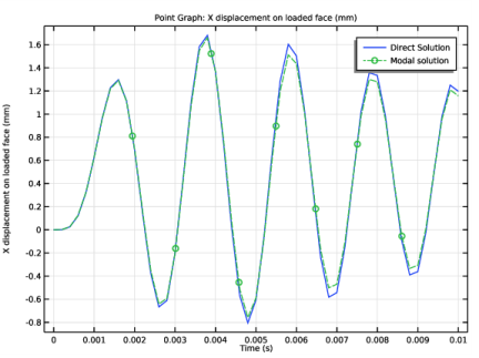
In the Settings window for 1D Plot Group, type Time-Dependent Displacement Graphs in the Label text field.
3
Locate the Data section. From the Dataset list, choose Time-Dependent Solution (sol4).
Point Graph 1
1
Right-click Time-Dependent Displacement Graphs and choose Point Graph.
2
3
In the Settings window for Point Graph, click Replace Expression in the upper-right corner of the y-Axis Data section. From the menu, choose Component 1 (comp1)>Solid Mechanics>Displacement>Displacement field - m>u - Displacement field, X component.
4
Locate the y-Axis Data section. From the Unit list, choose mm.
5
Select the Description check box.
6
In the associated text field, type X displacement on loaded face.
Study 4 (Time-Dependent)
Step 1: Time Dependent
1
In the Model Builder window, under Study 4 (Time-Dependent) click Step 1: Time Dependent.
2
In the Settings window for Time Dependent, click to expand the Results While Solving section.
3
Select the Plot check box.
4
From the Plot group list, choose Time-Dependent Displacement Graphs.
Solid Mechanics (solid)
A new load is needed for this study. You could just change the existing one, but when you have multiple studies it is better to have individual load nodes in the model tree and disable the ones not currently used in the study.
1
In the Model Builder window, expand the Component 1 (comp1) node.
Static Load
1
In the Model Builder window, expand the Solid Mechanics (solid) node, then click Boundary Load 1.
2
In the Settings window for Boundary Load, type Static Load in the Label text field.
Time-Dependent Load
1
In the Physics toolbar, click  Boundaries and choose Boundary Load.
2
In the Settings window for Boundary Load, type Time-Dependent Load in the Label text field.
3
4
Locate the Force section. Specify the FA vector as
Study 4 (Time-Dependent)
Step 1: Time Dependent
1
In the Model Builder window, under Study 4 (Time-Dependent) click Step 1: Time Dependent.
2
In the Settings window for Time Dependent, locate the Physics and Variables Selection section.
3
Select the Modify model configuration for study step check box.
4
In the tree, select Component 1 (Comp1)>Solid Mechanics (Solid)>Static Load.
5
Click  Disable.
6
In the Home toolbar, click  Compute.
Results
Time-Dependent Displacement Graphs
Compare the result for the x-displacement with the graph shown in Figure 7.
Since a plot was added manually, default plots are not created for this study. Copy, and modify, the existing stress plot.
Time-Dependent Stress Contour
1
In the Model Builder window, right-click Static Stress Contour and choose Duplicate.
2
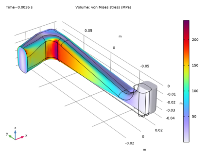
In the Settings window for 3D Plot Group, type Time-Dependent Stress Contour in the Label text field.
3
Locate the Data section. From the Dataset list, choose Time-Dependent Solution (sol4).
4
From the Time (s) list, choose 0.0036.
5
In the Time-Dependent Stress Contour toolbar, click  Plot.
Generate an animation of the solution.
Time-Dependent Stress Contour
1
In the Time-Dependent Stress Contour toolbar, click  Animation and choose Player.
2
In the Settings window for Animation, type Time-Dependent Stress Contour in the Label text field.
Time-Dependent Modal Analysis
In a modal-based analysis, the problem is reduced by representing the dynamics of the structure by a combination of a small number of its most significant eigenmodes. This is very efficient when the frequency content of the loads is limited, so that only a small number of modes are excited.
Results and Discussion
The plot in Figure 9 below shows the same x-displacement as in the previous section but with results from both the full and the modal based time-dependent analysis. The correspondence between the solutions is good even though only the first six eigenmodes are used.
Figure 9: x-displacement at a point on the loaded surface for full and modal analyses.
Figure 10 below shows the von Mises stress in the bracket at 0.0036 s. The maximum value is 233 MPa, which can be compared with the 238 MPa computed using the direct solution above. In general, more modes than what is needed to compute accurate displacements are required to obtain good stress solutions.
Figure 10: von Mises stress for modal solution.
Notes About the COMSOL Implementation
When you create a new study, it is possible to directly select Time Dependent, Modal. Such a study, however, generates a complete solver sequence including the eigenvalue computation step. Because the eigenvalues are already available, you create an Empty Study and add the study steps manually.
The undamped eigenmodes are used as the base, and the damping is provided by the material.
In the modal time-dependent procedure, all loads must have the same variation in time, specified in the study step. This means that you should not enter any time-dependent loads (that is, loads with an explicit dependency on the time variable t). If you are in a situation where all loads do not have the same temporal variation, you can instead use a more general approach available in the reduced order modeling framework.
Modeling Instructions
Add Study
1
In the Home toolbar, click  Add Study to open the Add Study window.
2
Go to the Add Study window.
3
Find the Studies subsection. In the Select Study tree, select Empty Study.
4
Click Add Study in the window toolbar.
5
In the Home toolbar, click  Add Study to close the Add Study window.
Solid Mechanics (solid)
Modal Time-Dependent Load
1
In the Physics toolbar, click  Boundaries and choose Boundary Load.
2
In the Settings window for Boundary Load, type Modal Time-Dependent Load in the Label text field.
3
4
Locate the Force section. Specify the FA vector as
Study 5 (Modal Time-Dependent)
1
In the Model Builder window, click Study 5.
2
In the Settings window for Study, type Study 5 (Modal Time-Dependent) in the Label text field.
Time Dependent, Modal
1
In the Study toolbar, click  Study Steps and choose Time Dependent>Time Dependent, Modal.
2
In the Settings window for Time Dependent, Modal, locate the Study Settings section.
3
In the Output times text field, type range(0,2e-4,10e-3).
4
Locate the Physics and Variables Selection section. Select the Modify model configuration for study step check box.
5
In the tree, select Component 1 (Comp1)>Solid Mechanics (Solid)>Static Load and Component 1 (Comp1)>Solid Mechanics (Solid)>Time-Dependent Load.
6
Click  Disable.
Solution, Modal Time-Dependent
1
In the Study toolbar, click  Show Default Solver.
2
In the Settings window for Solution, type Solution, Modal Time-Dependent in the Label text field.
3
In the Model Builder window, expand the Study 5 (Modal Time-Dependent)>Solver Configurations>Solution, Modal Time-Dependent (sol5) node, then click Modal Solver 1.
4
In the Settings window for Modal Solver, click to expand the Absolute Tolerance section.
5
From the Tolerance method list, choose Manual.
6
In the Absolute tolerance text field, type 1e-5.
7
Locate the Eigenpairs section. From the Solution list, choose Solution, Eigenfrequency (sol2).
8
Click to expand the Advanced section. In the Load factor text field, type 1+sin(2*pi*500[Hz]*t-pi/2).
9
In the Study toolbar, click  Compute.
Results
Modal Time-Dependent Solution
1
In the Model Builder window, under Results>Datasets click Study 5 (Modal Time-Dependent)/Solution, Modal Time-Dependent (sol5).
2
In the Settings window for Solution, type Modal Time-Dependent Solution in the Label text field.
Reproduce the plot in Figure 10 by following these instructions:
Modal Time-Dependent Stress Contour
1
In the Model Builder window, under Results click Stress (solid).
2
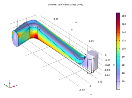
In the Settings window for 3D Plot Group, type Modal Time-Dependent Stress Contour in the Label text field.
3
Locate the Data section. From the Time (s) list, choose 0.0036.
Volume 1
1
In the Model Builder window, expand the Modal Time-Dependent Stress Contour node, then click Volume 1.
2
In the Settings window for Volume, locate the Expression section.
3
From the Unit list, choose MPa.
4
In the Modal Time-Dependent Stress Contour toolbar, click  Plot.
Add the results from this study to the graph of the direct time dependent results, so that the methods can be compared.
Point Graph 1
1
In the Model Builder window, under Results>Time-Dependent Displacement Graphs click Point Graph 1.
2
In the Settings window for Point Graph, click to expand the Legends section.
3
Select the Show legends check box.
4
From the Legends list, choose Manual.
5
Point Graph 2
1
Right-click Results>Time-Dependent Displacement Graphs>Point Graph 1 and choose Duplicate.
2
In the Settings window for Point Graph, locate the Data section.
3
From the Dataset list, choose Modal Time-Dependent Solution (sol5).
4
Click to expand the Coloring and Style section. Find the Line style subsection. From the Line list, choose Dashed.
5
Find the Line markers subsection. From the Marker list, choose Circle.
6
Locate the Legends section. In the table, enter the following settings:
7
Click to expand the Title section. From the Title type list, choose None.
In the Time-Dependent Displacement Graphs toolbar, click  Plot.
Frequency Response Analysis
A frequency response analysis solves for the linearized steady-state response from harmonic excitation loads. The loads can have amplitudes and phase shifts that depend on the excitation frequency, f:
where F(f) is the amplitude and FPh(f) is the phase shift of the load.
The result of a frequency response analysis is a complex time-dependent displacement field, which can be interpreted as an amplitude, uamp, and a phase angle, uphase. The actual displacement at any point in time is the real part of the solution
You can visualize the amplitudes and phases as well as the solution at a specific angle (time). When plotting, COMSOL Multiphysics multiplies the solution by , where is the angle specified in the Solution at angle (phase) text field in the settings for the dataset. The plot then shows the real part of the evaluated expression
The angle is available as the variable phase (radians) and can be used in plot expressions.
The purpose of this analysis is to find the response from a harmonic load with an excitation frequency in the range 350–650 Hz, which includes the first two eigenfrequencies found in the eigenfrequency analysis. The load amplitudes are
and there is no phase shift between the load components.
Results and Discussion
The amplitudes of the x-, y-, and z-displacements as functions of excitation frequency, at a point on the face where the load is applied, appear in the following figure:
Figure 11: Displacement amplitudes vs. excitation frequency.
The peaks in the displacement amplitude curves are associated with the two lowest eigenfrequencies of the bracket. Note that the lowest eigenfrequency, 416 Hz, corresponds to the peak on the x-displacement amplitude curve, while the next eigenfrequency, 573 Hz, corresponds to the peak on the z-displacement amplitude curve. This can be expected based on the eigenmode shapes obtained in the eigenfrequency analysis.
In Figure 12, the default stress plot is shown. For a frequency domain analysis, it shows the maximum von Mises stress in each point during the cycle.
Figure 12: Maximum equivalent stress during the cycle at the last frequency, 650 Hz-
Notes About the COMSOL Implementation
The loads are given without explicit time dependencies, since the harmonic variation is an underlying assumption in this analysis type. The loads can have different phase angles. This can either be obtained by adding a Phase subnode under the load, or by writing the load on a complex form.
Usually, when performing a frequency response analysis, you want to sweep over a frequency range. This can be done using the parametric solver, using the frequency as a parameter.
Modeling Instructions
Applied Loads (solid)
In the Model Builder window, under Results right-click Applied Loads (solid) and choose Delete.
Add Study
1
In the Home toolbar, click  Add Study to open the Add Study window.
2
Go to the Add Study window.
3
Find the Studies subsection. In the Select Study tree, select General Studies>Frequency Domain.
4
Click Add Study in the window toolbar.
5
In the Home toolbar, click  Add Study to close the Add Study window.
Study 6 (Frequency Domain)
1
In the Model Builder window, click Study 6.
2
In the Settings window for Study, type Study 6 (Frequency Domain) in the Label text field.
Step 1: Frequency Domain
1
In the Model Builder window, under Study 6 (Frequency Domain) click Step 1: Frequency Domain.
2
In the Settings window for Frequency Domain, locate the Study Settings section.
3
In the Frequencies text field, type range(350,10,650).
The load is the same as in the stationary study, so you can reuse the first load in the model tree.
4
Locate the Physics and Variables Selection section. Select the Modify model configuration for study step check box.
5
In the tree, select Component 1 (Comp1)>Solid Mechanics (Solid)>Time-Dependent Load and Component 1 (Comp1)>Solid Mechanics (Solid)>Modal Time-Dependent Load.
6
Click  Disable.
7
In the Home toolbar, click  Compute.
Solution, Frequency Domain
1
In the Model Builder window, expand the Study 6 (Frequency Domain)>Solver Configurations node, then click Solution 6 (sol6).
2
In the Settings window for Solution, type Solution, Frequency Domain in the Label text field.
Results
Frequency Domain Solution
1
In the Model Builder window, under Results>Datasets click Study 6 (Frequency Domain)/Solution, Frequency Domain (sol6).
2
In the Settings window for Solution, type Frequency Domain Solution in the Label text field.
Frequency-Response Stress Contour
1
In the Model Builder window, under Results click Stress (solid).
2
In the Settings window for 3D Plot Group, type Frequency-Response Stress Contour in the Label text field.
Volume 1
1
In the Model Builder window, expand the Frequency-Response Stress Contour node, then click Volume 1.
2
In the Settings window for Volume, locate the Expression section.
3
From the Unit list, choose MPa.
4
In the Frequency-Response Stress Contour toolbar, click  Plot.
Add a 1D plot group and reproduce the displacement amplitude graphs in Figure 11.
Applied Loads (solid)
In the Model Builder window, under Results right-click Applied Loads (solid) and choose Delete.
Frequency Response Displacement Graphs
1
In the Home toolbar, click  Add Plot Group and choose 1D Plot Group.
2
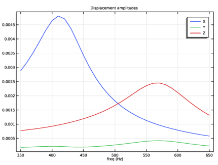
In the Settings window for 1D Plot Group, type Frequency Response Displacement Graphs in the Label text field.
3
Locate the Data section. From the Dataset list, choose Frequency Domain Solution (sol6).
4
Click to expand the Title section. From the Title type list, choose Manual.
5
In the Title text area, type Displacement amplitudes.
Point Graph 1
1
Right-click Frequency Response Displacement Graphs and choose Point Graph.
2
3
In the Settings window for Point Graph, click Replace Expression in the upper-right corner of the y-Axis Data section. From the menu, choose Component 1 (comp1)>Solid Mechanics>Displacement>Displacement amplitude (material and geometry frames) - m>solid.uAmpX - Displacement amplitude, X component.
4
Locate the Legends section. Select the Show legends check box.
5
From the Legends list, choose Manual.
6
Point Graph 2
1
Right-click Point Graph 1 and choose Duplicate.
2
In the Settings window for Point Graph, click Replace Expression in the upper-right corner of the y-Axis Data section. From the menu, choose Component 1 (comp1)>Solid Mechanics>Displacement>Displacement amplitude (material and geometry frames) - m>solid.uAmpY - Displacement amplitude, Y component.
3
Locate the Legends section. In the table, enter the following settings:
Point Graph 3
1
Right-click Point Graph 2 and choose Duplicate.
2
In the Settings window for Point Graph, click Replace Expression in the upper-right corner of the y-Axis Data section. From the menu, choose Component 1 (comp1)>Solid Mechanics>Displacement>Displacement amplitude (material and geometry frames) - m>solid.uAmpZ - Displacement amplitude, Z component.
3
Locate the Legends section. In the table, enter the following settings:
4
In the Frequency Response Displacement Graphs toolbar, click  Plot.
Compare the resulting plot with that in Figure 11.
Frequency Response Modal Analysis
You can also solve the same frequency response problem using the modal superposition method. The same remarks as for the time-dependent modal analysis above are relevant.
Results and Discussion
In Figure 13 below, the results from the modal frequency response analysis are overlaid on the results from the previous direct frequency response analysis (see Figure 11). The curves are almost indistinguishable. The response is to a large degree controlled by the lowest eigenmodes, which are used in the modal analysis. The modal method is however much more efficient in terms of computer resources.
Figure 13: Displacement amplitudes vs. excitation frequency for direct and modal frequency-response analyses.
Modeling Instructions
Solid Mechanics (solid)
Modal Frequency Load
1
In the Physics toolbar, click  Boundaries and choose Boundary Load.
2
In the Settings window for Boundary Load, type Modal Frequency Load in the Label text field.
3
Right-click Modal Frequency Load and choose Harmonic Perturbation.
The modal frequency response is a perturbation type of analysis. The load must then be declared as a perturbation load.
4
5
Locate the Force section. Specify the FA vector as
Add Study
1
In the Home toolbar, click  Add Study to open the Add Study window.
2
Go to the Add Study window.
3
Find the Studies subsection. In the Select Study tree, select Empty Study.
4
Click Add Study in the window toolbar.
5
In the Home toolbar, click  Add Study to close the Add Study window.
Study 7 (Modal Frequency Response)
In the Settings window for Study, type Study 7 (Modal Frequency Response) in the Label text field.
Frequency Domain, Modal
1
In the Study toolbar, click  Study Steps and choose Frequency Domain>Frequency Domain, Modal.
2
In the Settings window for Frequency Domain, Modal, locate the Study Settings section.
3
In the Frequencies text field, type range(350,10,650).
Since only loads having a harmonic perturbation are used in this study type, only the last added load, which is declared as a perturbation load, will be taken into account. For clarity, you can still disable all other loads.
4
Locate the Physics and Variables Selection section. Select the Modify model configuration for study step check box.
5
In the tree, select Component 1 (Comp1)>Solid Mechanics (Solid)>Static Load, Component 1 (Comp1)>Solid Mechanics (Solid)>Time-Dependent Load, and Component 1 (Comp1)>Solid Mechanics (Solid)>Modal Time-Dependent Load.
6
Click  Disable.
Solution, Modal Frequency-Domain
1
In the Study toolbar, click  Show Default Solver.
2
In the Settings window for Solution, type Solution, Modal Frequency-Domain in the Label text field.
3
In the Model Builder window, expand the Study 7 (Modal Frequency Response)>Solver Configurations>Solution, Modal Frequency-Domain (sol7) node, then click Modal Solver 1.
4
In the Settings window for Modal Solver, locate the Eigenpairs section.
5
From the Solution list, choose Solution, Eigenfrequency (sol2).
6
In the Study toolbar, click  Compute.
Results
Modal Frequency-Domain Solution
1
In the Model Builder window, under Results>Datasets click Study 7 (Modal Frequency Response)/Solution, Modal Frequency-Domain (sol7).
2
In the Settings window for Solution, type Modal Frequency-Domain Solution in the Label text field.
Modal Frequency-Response Stress Contour
1
In the Model Builder window, under Results click Stress (solid).
2
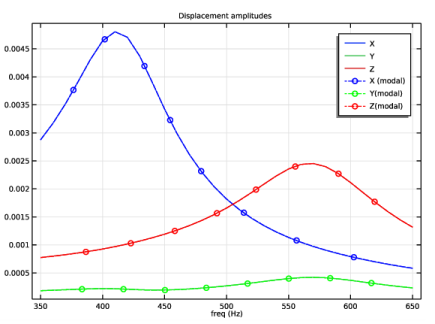
In the Settings window for 3D Plot Group, type Modal Frequency-Response Stress Contour in the Label text field.
Volume 1
1
In the Model Builder window, expand the Modal Frequency-Response Stress Contour node, then click Volume 1.
2
In the Settings window for Volume, locate the Expression section.
3
From the Unit list, choose MPa.
4
In the Modal Frequency-Response Stress Contour toolbar, click  Plot.
Reproduce the plot in Figure 13 as follows:
Point Graph 4
1
In the Model Builder window, under Results>Frequency Response Displacement Graphs right-click Point Graph 1 and choose Duplicate.
2
In the Settings window for Point Graph, locate the Data section.
3
From the Dataset list, choose Modal Frequency-Domain Solution (sol7).
4
Locate the Coloring and Style section. From the Color list, choose Blue.
5
Find the Line style subsection. From the Line list, choose Dashed.
6
Find the Line markers subsection. From the Marker list, choose Circle.
7
Locate the Legends section. In the table, enter the following settings:
Point Graph 5
1
Right-click Point Graph 4 and choose Duplicate.
2
In the Settings window for Point Graph, click Replace Expression in the upper-right corner of the y-Axis Data section. From the menu, choose Component 1 (comp1)>Solid Mechanics>Displacement>Displacement amplitude (material and geometry frames) - m>solid.uAmpY - Displacement amplitude, Y component.
3
Locate the Coloring and Style section. From the Color list, choose Green.
4
Locate the Legends section. In the table, enter the following settings:
Point Graph 6
1
Right-click Point Graph 5 and choose Duplicate.
2
In the Settings window for Point Graph, click Replace Expression in the upper-right corner of the y-Axis Data section. From the menu, choose Component 1 (comp1)>Solid Mechanics>Displacement>Displacement amplitude (material and geometry frames) - m>solid.uAmpZ - Displacement amplitude, Z component.
3
Locate the Coloring and Style section. From the Color list, choose Red.
4
Locate the Legends section. In the table, enter the following settings:
5
In the Frequency Response Displacement Graphs toolbar, click  Plot.
Parametric Analysis
A parametric analysis solves for the response as a function of a parameter. You can freely define the parameter name and what it affects; it can be a material property, a load parameter, or some other expression.
The purpose of this example is to find the response to static loading of the bracket as a function of the direction of the load parameterized by the angle α.
Apply the load on the face shown in Figure 2. To control the direction of the load, introduce a parameter in the load expressions:
where α is the angle of the load direction in the xz-plane. Let 45°≤ α≤ 45°. 
Results and Discussion
The following plot shows the x-, y-, and z-displacements as functions of the direction of the load, α, at a point on the surface where the load is applied:
Figure 14: Displacement amplitudes versus load direction.
Notes About the COMSOL Implementation
When you perform a parametric study, you will select the underlying study type (here: Stationary) first. Then you add a Parametric feature, and define the parameter values.
Modeling Instructions
Applied Loads (solid)
In the Model Builder window, under Results right-click Applied Loads (solid) and choose Delete.
Add Study
1
In the Home toolbar, click  Add Study to open the Add Study window.
2
Go to the Add Study window.
3
Find the Studies subsection. In the Select Study tree, select General Studies>Stationary.
4
Click Add Study in the window toolbar.
5
In the Home toolbar, click  Add Study to close the Add Study window.
Study 8 (Parametric Static)
1
In the Model Builder window, click Study 8.
2
In the Settings window for Study, type Study 8 (Parametric Static) in the Label text field.
Parametric Sweep
In the Study toolbar, click  Parametric Sweep.
It is necessary to define the parameters to be used. The values given here do not influence the parametric solver, but can be used for studies outside it.
Global Definitions
Parameters 1
1
In the Model Builder window, under Global Definitions click Parameters 1.
2
In the Settings window for Parameters, locate the Parameters section.
3
Add a load with a parameter dependency.
Solid Mechanics (solid)
Parametric Load
1
In the Physics toolbar, click  Boundaries and choose Boundary Load.
2
In the Settings window for Boundary Load, type Parametric Load in the Label text field.
3
4
Locate the Force section. Specify the FA vector as
Study 8 (Parametric Static)
Parametric Sweep
1
In the Model Builder window, under Study 8 (Parametric Static) click Parametric Sweep.
2
In the Settings window for Parametric Sweep, locate the Study Settings section.
3
4
Step 1: Stationary
1
In the Model Builder window, click Step 1: Stationary.
2
In the Settings window for Stationary, locate the Physics and Variables Selection section.
3
Select the Modify model configuration for study step check box.
4
In the tree, select Component 1 (Comp1)>Solid Mechanics (Solid)>Static Load, Component 1 (Comp1)>Solid Mechanics (Solid)>Time-Dependent Load, Component 1 (Comp1)>Solid Mechanics (Solid)>Modal Time-Dependent Load, and Component 1 (Comp1)>Solid Mechanics (Solid)>Modal Frequency Load.
5
Click  Disable.
6
In the Home toolbar, click  Compute.
Solution, Parametric Static
1
In the Model Builder window, expand the Study 8 (Parametric Static)>Solver Configurations node, then click Solution 8 (sol8).
2
In the Settings window for Solution, type Solution, Parametric Static in the Label text field.
Results
Parametric Static Solution
1
In the Model Builder window, under Results>Datasets click Study 8 (Parametric Static)/Solution, Parametric Static (sol8).
2
In the Settings window for Solution, type Parametric Static Solution in the Label text field.
Stress (solid)
In the Model Builder window, under Results right-click Stress (solid) and choose Delete.
Applied Loads, Parametric Solution
1
In the Model Builder window, under Results click Applied Loads (solid).
2
In the Settings window for Group, type Applied Loads, Parametric Solution in the Label text field.
3
In the Model Builder window, expand the Applied Loads, Parametric Solution node.
Boundary Loads (solid) 1
In the Model Builder window, expand the Results>Applied Loads, Parametric Solution>Boundary Loads (solid) 1 node.
Transparency 1
1
In the Model Builder window, expand the Results>Applied Loads, Parametric Solution>Boundary Loads (solid) 1>Gray Surfaces node.
2
Right-click Transparency 1 and choose Disable.
Results
Applied Loads, Parametric Solution
1
In the Model Builder window, collapse the Results>Applied Loads, Parametric Solution node.
2
In the Model Builder window, click Results.
3
Click Yes to confirm.
Parametric Response Graphs
1
In the Home toolbar, click  Add Plot Group and choose 1D Plot Group.
2
In the Settings window for 1D Plot Group, type Parametric Response Graphs in the Label text field.
3
Locate the Data section. From the Dataset list, choose Parametric Static Solution (sol8).
4
Locate the Title section. From the Title type list, choose None.
5
Locate the Plot Settings section. Select the x-axis label check box.
6
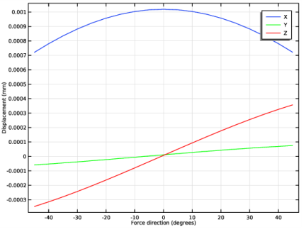
In the associated text field, type Force direction (degrees).
7
Select the y-axis label check box.
8
Point Graph 1
1
Right-click Parametric Response Graphs and choose Point Graph.
2
3
In the Settings window for Point Graph, locate the y-Axis Data section.
4
In the Expression text field, type u.
5
Locate the Legends section. Select the Show legends check box.
6
From the Legends list, choose Manual.
7
Point Graph 2
1
Right-click Point Graph 1 and choose Duplicate.
2
In the Settings window for Point Graph, locate the y-Axis Data section.
3
In the Expression text field, type v.
4
Locate the Coloring and Style section. From the Color list, choose Green.
5
Locate the Legends section. In the table, enter the following settings:
Point Graph 3
1
Right-click Point Graph 2 and choose Duplicate.
2
In the Settings window for Point Graph, locate the y-Axis Data section.
3
In the Expression text field, type w.
4
Locate the Coloring and Style section. From the Color list, choose Red.
5
Locate the Legends section. In the table, enter the following settings:
In the Parametric Response Graphs toolbar, click  Plot.
Linear Buckling Analysis
A structure under compression can sometimes become unstable due to buckling. The critical buckling load can be estimated using a linear buckling analysis.
To perform this analysis, you first run a stress analysis with an arbitrary load level. In a second study step, the buckling load is computed as a scale factor with respect to the load used in the first analysis.
Results and Discussion
The computed eigenvalue is 103. Since the load applied in the stationary step was 1 kN, the estimated buckling load is 103 kN. The shape of the buckling mode is shown below.
Figure 15: Buckling mode shape.
It can be noted that the stresses caused by the preload are so large in this structure that a plastic collapse would occur long before the buckling load was reached.
Notes About the COMSOL Implementation
When a Linear Buckling study is selected, both study steps are automatically prepared. It is only necessary to define the reference load.
Modeling Instructions
Add Study
1
In the Home toolbar, click  Add Study to open the Add Study window.
2
Go to the Add Study window.
3
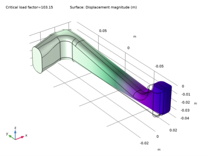
Find the Studies subsection. In the Select Study tree, select Preset Studies for Selected Physics Interfaces>Linear Buckling.
4
Click Add Study in the window toolbar.
5
In the Home toolbar, click  Add Study to close the Add Study window.
Solid Mechanics (solid)
Next, set up the buckling preload.
Buckling Preload
1
In the Physics toolbar, click  Boundaries and choose Boundary Load.
2
In the Settings window for Boundary Load, type Buckling Preload in the Label text field.
3
4
Locate the Force section. From the Load type list, choose Total force.
5
Specify the Ftot vector as
Study 9 (Linear Buckling)
1
In the Model Builder window, click Study 9.
2
In the Settings window for Study, type Study 9 (Linear Buckling) in the Label text field.
Step 1: Stationary
1
In the Model Builder window, under Study 9 (Linear Buckling) click Step 1: Stationary.
2
In the Settings window for Stationary, locate the Physics and Variables Selection section.
3
Select the Modify model configuration for study step check box.
4
In the tree, select
Component 1 (Comp1)>Solid Mechanics (Solid)>Static Load,
Component 1 (Comp1)>Solid Mechanics (Solid)>Time-Dependent Load, Component 1 (Comp1)>Solid Mechanics (Solid)>Modal Time-Dependent Load, Component 1 (Comp1)>Solid Mechanics (Solid)>Modal Frequency Load, and Component 1 (Comp1)>Solid Mechanics (Solid)>Parametric Load.
5
Click  Disable.
Step 2: Linear Buckling
1
In the Model Builder window, click Step 2: Linear Buckling.
2
In the Settings window for Linear Buckling, locate the Physics and Variables Selection section.
3
Select the Modify model configuration for study step check box.
4
In the tree, select
Component 1 (Comp1)>Solid Mechanics (Solid)>Static Load,
Component 1 (Comp1)>Solid Mechanics (Solid)>Time-Dependent Load, Component 1 (Comp1)>Solid Mechanics (Solid)>Modal Time-Dependent Load, Component 1 (Comp1)>Solid Mechanics (Solid)>Modal Frequency Load, and Component 1 (Comp1)>Solid Mechanics (Solid)>Parametric Load.
5
Click  Disable.
6
In the Home toolbar, click  Compute.
Solution, Linear Buckling
1
In the Model Builder window, expand the Study 9 (Linear Buckling)>Solver Configurations node, then click Solution 9 (sol9).
2
In the Settings window for Solution, type Solution, Linear Buckling in the Label text field.
Results
Linear Buckling Solution
1
In the Model Builder window, under Results>Datasets click Study 9 (Linear Buckling)/Solution, Linear Buckling (sol9).
2
In the Settings window for Solution, type Linear Buckling Solution in the Label text field.
Linear Buckling Preload Solution
1
In the Model Builder window, under Results>Datasets click Study 9 (Linear Buckling)/Solution Store 1 (sol10).
2
In the Settings window for Solution, type Linear Buckling Preload Solution in the Label text field.
With the following steps you can reproduce the plot in Figure 15:
Surface 1
1
In the Model Builder window, expand the Mode Shape (solid) node, then click Surface 1.
2
In the Mode Shape (solid) toolbar, click  Plot.
Buckling Shape Plot
1
In the Model Builder window, under Results click Mode Shape (solid).
2
In the Settings window for 3D Plot Group, type Buckling Shape Plot in the Label text field.
Make all the studies possible to repeat by disabling loads which were added since each study was analyzed.
Study 1 (Static)
Step 1: Stationary
1
In the Model Builder window, expand the Study 1 (Static) node, then click Step 1: Stationary.
2
In the Settings window for Stationary, locate the Physics and Variables Selection section.
3
Select the Modify model configuration for study step check box.
4
In the tree, select
Component 1 (Comp1)>Solid Mechanics (Solid)>Time-Dependent Load, Component 1 (Comp1)>Solid Mechanics (Solid)>Modal Time-Dependent Load, Component 1 (Comp1)>Solid Mechanics (Solid)>Modal Frequency Load, Component 1 (Comp1)>Solid Mechanics (Solid)>Parametric Load, and Component 1 (Comp1)>Solid Mechanics (Solid)>Buckling Preload.
5
Click  Disable.
Study 4 (Time-Dependent)
Step 1: Time Dependent
1
In the Model Builder window, under Study 4 (Time-Dependent) click Step 1: Time Dependent.
2
In the Settings window for Time Dependent, locate the Physics and Variables Selection section.
3
In the tree, select
Component 1 (Comp1)>Solid Mechanics (Solid)>Modal Time-Dependent Load,
Component 1 (Comp1)>Solid Mechanics (Solid)>Modal Frequency Load, Component 1 (Comp1)>Solid Mechanics (Solid)>Parametric Load, and Component 1 (Comp1)>Solid Mechanics (Solid)>Buckling Preload.
4
Click  Disable.
Study 5 (Modal Time-Dependent)
Step 1: Time Dependent, Modal
1
In the Model Builder window, under Study 5 (Modal Time-Dependent) click Step 1: Time Dependent, Modal.
2
In the Settings window for Time Dependent, Modal, locate the Physics and Variables Selection section.
3
In the tree, select Component 1 (Comp1)>Solid Mechanics (Solid)>Modal Frequency Load, Component 1 (Comp1)>Solid Mechanics (Solid)>Parametric Load, and Component 1 (Comp1)>Solid Mechanics (Solid)>Buckling Preload.
4
Click  Disable.
Study 6 (Frequency Domain)
Step 1: Frequency Domain
1
In the Model Builder window, under Study 6 (Frequency Domain) click Step 1: Frequency Domain.
2
In the Settings window for Frequency Domain, locate the Physics and Variables Selection section.
3
In the tree, select Component 1 (Comp1)>Solid Mechanics (Solid)>Modal Frequency Load, Component 1 (Comp1)>Solid Mechanics (Solid)>Parametric Load, and Component 1 (Comp1)>Solid Mechanics (Solid)>Buckling Preload.
4
Click  Disable.
Study 7 (Modal Frequency Response)
Step 1: Frequency Domain, Modal
1
In the Model Builder window, under Study 7 (Modal Frequency Response) click Step 1: Frequency Domain, Modal.
2
In the Settings window for Frequency Domain, Modal, locate the Physics and Variables Selection section.
3
In the tree, select Component 1 (Comp1)>Solid Mechanics (Solid)>Parametric Load and Component 1 (Comp1)>Solid Mechanics (Solid)>Buckling Preload.
4
Click  Disable.
Study 8 (Parametric Static)
Step 1: Stationary
1
In the Model Builder window, under Study 8 (Parametric Static) click Step 1: Stationary.
2
In the Settings window for Stationary, locate the Physics and Variables Selection section.
3
In the tree, select Component 1 (Comp1)>Solid Mechanics (Solid)>Buckling Preload.
4
Click  Disable.