Vibrating String

PDF

Vibrating String

In the following example you compute the natural frequencies of a pretensioned string using the 2D Truss interface. This is an example of “stress stiffening”. In fact the transverse stiffness of truss elements is directly proportional to the tensile force.

Strings made of piano wire have an extremely high yield limit, thus enabling a wide range of pretension forces.

The results are compared with the analytical solution.

Model Definition

The finite element idealization consists of a single line. The diameter of the wire is irrelevant for the solution of this particular problem, but it must still be given.

•

String length, L = 0.5 m

•

Cross section diameter 1.0 mm; A = 0.785 mm2

•

Young’s modulus, E = 210 GPa

•

Poisson’s ratio, ν = 0.31

•

Mass density, ρ = 7850 kg/m3

Both ends of the wire are fixed.

The wire is pretensioned to σni = 1520 MPa.

Results and Discussion

The analytical solution for the natural frequencies of the vibrating string (Ref. 1) is

(1)

The pretensioning stress σni in this example is tuned so that the first natural frequency is Concert A; 440 Hz.

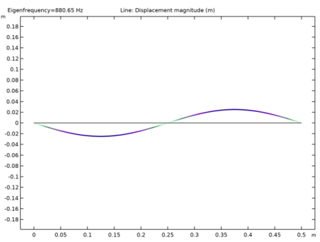
In Table 1 the computed results are compared with the results from Equation 1. The agreement is very good. The accuracy decreases with increasing complexity of the mode shape, because the possibility for the relatively coarse mesh to describe such a shape is limited. The mode shapes for the first three modes are shown in Figure 1 through Figure 3.

Table 1: Comparison between analytical and computed natural frequencies.
Mode number	Analytical frequency (Hz)	COMSOL result (Hz)
1	440.0	440.1
2	880.0	880.6
3	1320	1322
4	1760	1765
5	2200	2209

Figure 1: First eigenmode.

Figure 2: Second eigenmode.

Figure 3: Third eigenmode.

Notes About the COMSOL Implementation

In this example, the stresses are known in advance, so it is possible to use an initial stress condition. This is shown in the first study.

In a general case, the prestress is given by some external loading. The structural response of to this loading needs to be calculated and incorporated into the structure before the eigenfrequency can be computed. Such a study therefore consists of two steps: One stationary step for computing the prestressed state, and one step for the eigenfrequency. The special study type Prestressed Analysis, Eigenfrequency can be used to set up such a sequence. This is shown in the second study in this example.

Since an unstressed string has no stiffness in the transverse direction, it is generally difficult to get an analysis to converge without taking special measures. One such method is shown in the second study: A spring foundation is added during initial loading, and is then removed.

You must switch on geometrical nonlinearity in the study in order to capture effects of prestress. This is done automatically when a study of the type Prestressed Analysis, Eigenfrequency is used.

1. R. Knobel, An Introduction to the Mathematical Theory of Waves, The American Mathematical Society, 2000.

Structural_Mechanics_Module/Verification_Examples/vibrating_string

Modeling Instructions

From the menu, choose .

In the window, click

.

1

In the window, click

.

2

In the tree, select .

3

4

5

In the tree, select .

6

Polygon 1 (pol1)

1

In the toolbar, click

.

2

In the window for , locate the section.

3

In the table, enter the following settings:


x (m)	y (m)
0	0
0.5	0

4

.

Material 1 (mat1)

1

In the window, under right-click and choose .

2

In the window for , locate the section.

3

In the table, enter the following settings:


Property	Variable	Value	Unit	Property group
Young’s modulus	E	210e9	Pa	Young’s modulus and Poisson’s ratio
Poisson’s ratio	nu	0.31	1	Young’s modulus and Poisson’s ratio
Density	rho	7850	kg/m³	Basic

Cross-Section Data 1

1

In the window, under click .

2

In the window for , locate the section.

3

In the A text field, type pi/4*0.001^2.

1

In the toolbar, click

and choose .

2

In the window for , locate the section.

3

From the list, choose .

The straight edge constraint must be removed because the vibration gives the string a curved shape.

Linear Elastic Material 1

In the window, click .

Initial Stress and Strain 1

1

In the toolbar, click

and choose .

2

In the window for , locate the section.

3

In the σn0 text field, type 1520e6.

1

In the toolbar, click

.

2

In the window for , locate the section.

3

From the list, choose .

1

In the window, click .

2

In the window for , locate the section.

3

Click the button.

4

Locate the section. In the text field, type 0.01.

This setting results in a mesh with 50 elements, which COMSOL Multiphysics generates when you solve the model.

The stiffness caused by the prestress is a nonlinear effect, so geometric nonlinearity must be switched on.

Step 1: Eigenfrequency

1

In the window, under click .

2

In the window for , locate the section.

3

Find the subsection. Select the check box.

4

In the toolbar, click

.

Mode Shape (truss)

1

button in the toolbar.

The default plot shows the displacement for the first eigenmode.

1

In the window, expand the node, then click .

2

In the window for , locate the section.

3

In the text field, type 2.

Mode Shape (truss)

1

button in the toolbar.

2

In the window, click .

3

In the window for , locate the section.

4

From the list, choose .

This corresponds to the second eigenmode.

5

In the toolbar, click

.

6

button in the toolbar.

7

From the list, choose .

This is the third eigenmode.

8

In the toolbar, click

.

9

button in the toolbar.

Now, prepare a second study where the prestress is instead computed from an external load. The pinned condition at the right end must then be replaced by a force.

1

In the toolbar, click

and choose .

2

Select Point 1 only.

Prescribed Displacement 1

1

In the toolbar, click

and choose .

2

Select Point 2 only.

3

In the window for , locate the section.

4

Select the check box.

1

In the toolbar, click

and choose .

2

Select Point 2 only.

3

In the window for , locate the section.

4

Specify the FP vector as


1520[MPa]*truss.area	x
0	y

Add a spring with an arbitrary, small stiffness in order to suppress the out-of-plane singularity of the unstressed wire.

Spring Foundation 1

1

In the toolbar, click

and choose .

2

Select Boundary 1 only.

3

In the window for , locate the section.

4

From the list, choose .

5

In the kL table, enter the following settings:


0	0
0	10

1

In the toolbar, click

to open the window.

2

Go to the window.

3

Find the subsection. In the tree, select .

4

Click in the window toolbar.

5

In the toolbar, click

to close the window.

Step 1: Stationary

Switch off the initial stress and double-sided pinned condition, which should not be part of the second study. In the eigenfrequency step, the stabilizing spring support must also be removed.

1

In the window for , locate the section.

2

Select the check box.

3

In the tree, select and .

4

Step 2: Eigenfrequency

1

In the window, click .

2

In the window for , locate the section.

3

Select the check box.

4

In the tree, select , , and .

5

6

In the toolbar, click

.

Mode Shape (truss) 1

The eigenfrequencies computed using this more general approach are close to those computed in the previous step.

1

In the window, expand the node, then click .

2

In the window for , locate the section.

3

In the text field, type 2.

To make behave as when it was first created, the features added for must be disabled.

Step 1: Eigenfrequency

1

In the window, under click .

2

In the window for , locate the section.

3

Select the check box.

4

In the tree, select , , , and .

5