|
|
|
|
•
|
A short version, elbow_bracket_brief, treating the three first analysis types in the above list.
|
|
•
|
A complete version, elbow_bracket, treating all nine analysis types.
|

|
1
|
|
2
|
|
3
|
Click Add.
|
|
4
|
Click
|
|
5
|
|
6
|
Click
|
|
1
|
|
2
|
|
3
|
|
4
|
Click
|
|
5
|
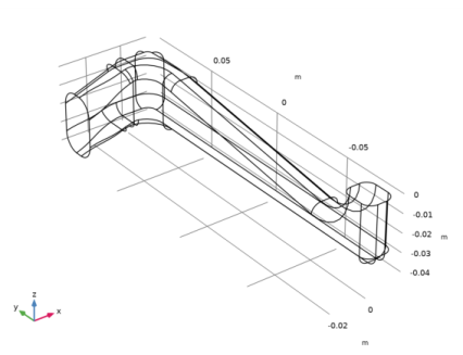
Browse to the model’s Application Libraries folder and double-click the file elbow_bracket.mphbin.
|
|
6
|
Click
|
|
7
|
|
8
|
Click the
|
|
1
|
|
2
|
On the object fin, select Edges 17, 21, 23, 27, 38, 40, 42, and 44 only.
|
|
1
|
|
2
|
|
3
|
|
4
|
|
6
|
|
1
|
|
2
|
|
3
|
|
4
|
|
1
|
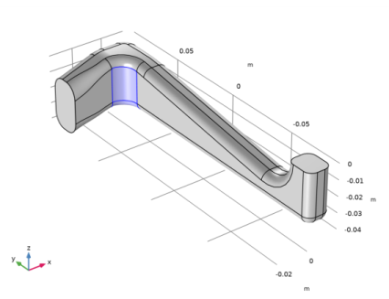
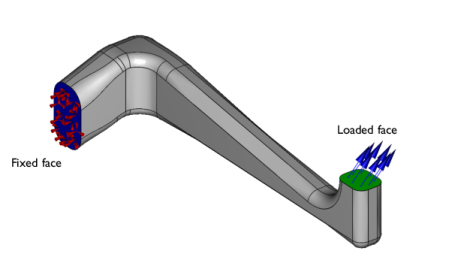
In the Model Builder window, under Component 1 (comp1) right-click Solid Mechanics (solid) and choose Fixed Constraint.
|
|
1
|
|
3
|
|
4
|
|
1
|
|
2
|
|
3
|
|
1
|
In the Model Builder window, expand the Study 1 (Static)>Solver Configurations node, then click Solution 1 (sol1).
|
|
2
|
|
1
|
In the Model Builder window, expand the Results>Datasets node, then click Study 1 (Static)/Solution, Static (sol1).
|
|
2
|
|
1
|
|
2
|
|
1
|
|
2
|
|
3
|
|
4
|
|
5
|
|
1
|
|
2
|
|
1
|
|
2
|
|
1
|
In the Model Builder window, under Results>Applied Loads, Static Solution click Boundary Loads (solid).
|
|
2
|
|
1
|
|
2
|
|
3
|
|
4
|
|
1
|
|
2
|
|
1
|
In the Model Builder window, under Study 1 (Static)>Solver Configurations right-click Solution, Static (sol1) and choose Solution>Update.
|
|
1
|
|
2
|
In the Settings window for Global Evaluation, click Replace Expression in the upper-right corner of the Expressions section. From the menu, choose Component 1 (comp1)>Definitions>Variables>U_max - Maximum deflection - m.
|
|
3
|
Locate the Expressions section. In the table, enter the following settings:
|
|
4
|
Click
|
|
1
|
|
2
|
|
1
|
|
2
|
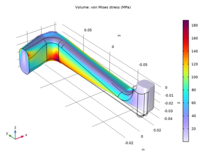
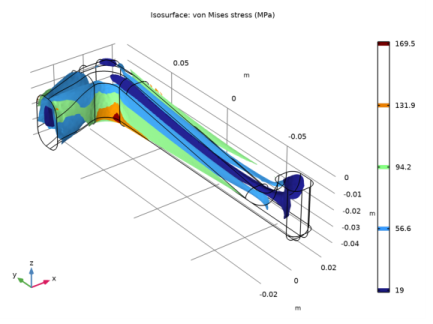
In the Settings window for Isosurface, click Replace Expression in the upper-right corner of the Expression section. From the menu, choose Component 1 (comp1)>Solid Mechanics>Stress>solid.mises - von Mises stress - N/m².
|
|
3
|
|
1
|
|
2
|
|
1
|
|
2
|
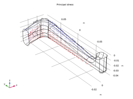
In the Settings window for 3D Plot Group, type Static Principal Stress Arrow Plot in the Label text field.
|
|
1
|
In the Static Principal Stress Arrow Plot toolbar, click
|
|
2
|
|
3
|
|
4
|
|
5
|
|
1
|
|
2
|
|
3
|
|
4
|
|
5
|
|
1
|
|
2
|
|
3
|
|
1
|
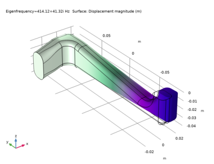
In the Model Builder window, expand the Study 2 (Eigenfrequency)>Solver Configurations node, then click Solution 2 (sol2).
|
|
2
|
|
1
|
In the Model Builder window, under Results>Datasets click Study 2 (Eigenfrequency)/Solution, Eigenfrequency (sol2).
|
|
2
|
|
1
|
|
2
|
|
3
|
|
4
|
|
5
|
|
1
|
In the Model Builder window, expand the Results>Undamped Mode Shapes node, then click Results>Export>Animation 1.
|
|
2
|
|
1
|
|
2
|
|
3
|
|
4
|
|
5
|
|
1
|
|
2
|
|
3
|
|
4
|
|
5
|
|
6
|
|
7
|
|
1
|
|
2
|
|
3
|
|
1
|
In the Model Builder window, expand the Study 3 (Damped Eigenfrequency)>Solver Configurations node, then click Solution 3 (sol3).
|
|
2
|
|
1
|
In the Model Builder window, under Results>Datasets click Study 3 (Damped Eigenfrequency)/Solution, Damped Eigenfrequency (sol3).
|
|
2
|
|
1
|
|
2
|
|
1
|
In the Model Builder window, expand the Damped Mode Shapes node, then click Study 2 (Eigenfrequency)>Step 1: Eigenfrequency.
|
|
2
|
|
3
|
|
4
|
In the tree, select Component 1 (Comp1)>Solid Mechanics (Solid)>Linear Elastic Material 1>Damping 1.
|
|
5
|
Click
|