PDF

Petzval Lens STOP Analysis with Hyperelasticity
Introduction
Many optical systems are required to be operated in extreme environments, where temperature changes are significant. This will invariably induce deformations in the optical geometry. In order to simulate the effects of structural and thermal deformation on the optical performance of a lens a structural-thermal-optical performance (STOP) analysis should be performed. In this tutorial an integrated STOP analysis is demonstrated.
The Petzval Lens STOP Analysis tutorial is used as the basis for this model. In that model a Petzval lens is modeled together with a simple barrel geometry (see Figure 1) and subjected to uniform temperature of 25°C. In these models, silicone RTV is assumed to be used to support the lens elements within the barrel. Because this is nominally a hyperelastic material, it would be more accurate to use a non-linear material model to compute the deformation of these supports. Such a model could be used together with surface-to-surface radiation to perform a parametric sweep over a range of material and/or other properties (for example, temperature). See Petzval Lens STOP Analysis with Surface-to-Surface Radiation and Petzval Lens STOP Analysis Isothermal Sweep for example models.
Figure 1: An overview of the Petzval Lens STOP analysis geometry. The lenses are shown in blue, the lens supports are colored red, and the detector assembly is dark gray. A simple barrel assembly connects these elements.
Model Definition
Details of the lens simulated in this tutorial can be found in the Petzval Lens tutorial (see Ref. 1, p. 191). For this model a simple barrel geometry and detector assembly has been added. The instructions for creating the geometry used in this model can be found in the appendix of Petzval Lens STOP Analysis.
Figure 2: The Petzval Lens Stop Analysis geometry sequence.
The default Neo-Hookean material model is used in the Hyperelastic Material interface, where the material is assumed to be incompressible. A Lamé parameter μ = 40 MPa is an average from data in Ref. 4. The material properties and all other details of the simulation remain unchanged.
Results and Discussion
As in Petzval Lens STOP Analysis, a ray trace is performed using three wavelengths (475 nm, 550 nm, and 625 nm) over three field angles (0°, 3.5°, and 7.0°). The resulting temperature, displacement, and von Mises stress fields are shown in Figure 3 and Figure 4.
The image quality on the nominal and “best focus” image planes is shown in Figure 5 and Figure 6. When compared with a model not using hyperelastic effects (that is, Petzval Lens STOP Analysis) it can be seen that the image planes are shifted by 3 μm and 2 μm when comparing the nominal and best focus image planes respectively. This suggests that the hyperelastic material properties have a small, but not insignificant impact on the model.
Figure 3: A ray trace shown together with a 3/4 section view of the Petzval lens assembly. The von Mises Stress field is on the cross-sections.
Figure 4: In this ray trace, the displacement field is shown together with the von Mises stress.
Figure 5: The image quality on the nominal image surface. This is the detector surface after being subject to thermal expansion.
Figure 6: Image quality on the best focus plane. That is, this is the surface that gives the minimum RMS spot size on-axis.
References
1. M.J. Kidger, Fundamental Optical Design, Bellingham WA, USA: SPIE Press, 2001.
2. https://www.us.schott.com/english/index.html.
3. http://www.oharacorp.com/catalog.html.
4. M.A. Salama, W.M. Rowe, and R.K. Yasui, “Thermoelatic Analysis of Solar Cell Arrays and their Material Properties,” Technical Memorandum 33-626, NASA, 1973.
5. T.M. Mower, “Thermomechanical behavior of aerospace-grade RTV (silicone adhesive).” International Journal of Adhesions and Adhesives 87 (2018): 64-72.
6. P.R. Yoder, Jr., Opto-Mechanical Systems Design, Bellingham WA, USA: SPIE Press, 2006.
Application Library path: Ray_Optics_Module/Structural_Thermal_Optical_Performance_Analysis/petzval_lens_stop_analysis_with_hyperelasticity
Modeling Instructions
Application Libraries
1
From the File menu, choose Application Libraries.
2
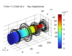
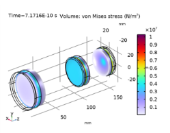
In the Application Libraries window, select Ray Optics Module>Structural Thermal Optical Performance Analysis>petzval_lens_stop_analysis in the tree.
3
Component 1 (comp1)
The instructions for creating the geometry in the appendix of the Petzval Lens STOP analysis tutorial. Orient the view to match Figure 2.
Add the Hyperelastic Material interface and select the lens supports.
1
In the Model Builder window, expand the Component 1 (comp1) node.
Solid Mechanics (solid)
Hyperelastic Material 1
1
In the Model Builder window, expand the Component 1 (comp1)>Solid Mechanics (solid) node.
2
Right-click Solid Mechanics (solid) and choose Material Models>Hyperelastic Material.
3
In the Settings window for Hyperelastic Material, locate the Domain Selection section.
4
From the Selection list, choose Supports.
5
Locate the Hyperelastic Material section. From the Compressibility list, choose Incompressible material.
6
From the μ list, choose User defined. In the associated text field, type 40[MPa].
Thermal Expansion 1
1
In the Physics toolbar, click  Attributes and choose Thermal Expansion.
2
In the Home toolbar, click  Compute.
Results
Ray Trajectories (gop)
The Ray Trajectories plot and the Stress plots (see below) are created by default with this combination of physics and study steps.
Stress (solid)
Temperature
Click the  Zoom Extents button in the Graphics toolbar. The result should match Figure 3.
Displacement
Click the  Zoom Extents button in the Graphics toolbar. The result should look like Figure 4.
Spot Diagram, Nominal
Click the  Zoom Extents button in the Graphics toolbar. The nominal image surface spot diagram should look like Figure 5.
Spot Diagram 1
1
In the Model Builder window, under Results>Spot Diagram, Best Focus click Spot Diagram 1.
2
In the Settings window for Spot Diagram, locate the Filters section.
3
Select the Filter by release feature index check box.
4
Click to expand the Focal Plane Orientation section. Click Recompute Focal Plane Dataset.
5
Locate the Filters section. Clear the Filter by release feature index check box.
6
In the Spot Diagram, Best Focus toolbar, click  Plot.
7
Click the  Zoom Extents button in the Graphics toolbar. The best focus spot diagram should look like Figure 6.