
|
|
|
|
-56.9 μm
|
72.5 μm
|
|
|
-25.3 μm
|
31.4 μm
|
|
|
6.3 μm
|
-9.4 μm
|
|
|
37.9 μm
|
-50.3 μm
|
|
1
|
|
2
|
In the Application Libraries window, select Ray Optics Module>Structural Thermal Optical Performance Analysis>petzval_lens_stop_analysis in the tree.
|
|
3
|
Click
|
|
1
|
|
2
|
|
3
|
|
4
|
|
1
|
|
2
|
|
3
|
Click
|
|
5
|
|
1
|
|
2
|
|
3
|
|
1
|
|
2
|
|
3
|
From the Solution list, choose Parametric Solutions 1 (sol3). This is the solution dataset for the parametric sweep.
|
|
1
|
|
2
|
|
3
|
|
5
|
|
7
|
|
9
|
|
1
|
|
2
|
|
3
|
|
5
|
|
7
|
|
9
|
|
1
|
|
2
|
|
3
|
|
4
|
|
5
|
Locate the Extra Time Steps section. From the Maximum number of extra time steps rendered list, choose All.
|
|
1
|
|
2
|
|
3
|
|
1
|
|
2
|
|
3
|
|
1
|
|
2
|
|
3
|
|
1
|
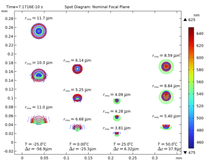
In the Model Builder window, expand the Results>Spot Diagram, Nominal node, then click Spot Diagram 1.
|
|
2
|
|
3
|
|
4
|
|
1
|
|
2
|
|
3
|
|
4
|
|
5
|
|
1
|
|
2
|
|
3
|
|
4
|
|
1
|
|
2
|
|
3
|
|
4
|
|
1
|
|
2
|
|
3
|
|
4
|
|
5
|
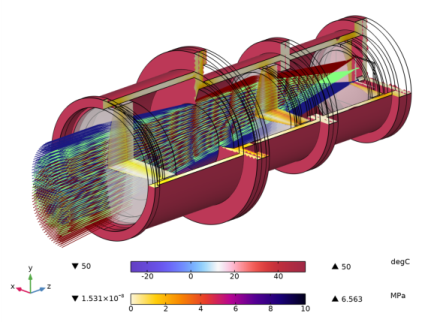
Locate the Annotation section. In the Text text field, type $T = eval(T0-0[degC])^\circ$C \\ $\Delta z = eval((aveop1(z)-z_image)/1[um])\,\unicode{\mu}$m. The position of the undeformed image plane is z_image.
|
|
6
|
|
7
|
|
8
|
|
9
|
|
10
|
|
11
|
|
1
|
|
2
|
|
3
|
|
4
|
|
1
|
|
2
|
|
3
|
|
4
|
|
1
|
|
2
|
|
3
|
|
4
|
|
5
|
|
1
|
|
2
|
|
3
|
|
4
|
|
1
|
|
2
|
|
3
|
|
1
|
|
2
|
|
3
|
|
1
|
|
2
|
|
3
|
|
1
|
|
2
|
|
3
|
|
4
|
Click to collapse the Layout section. Locate the Annotations section. Clear the Show spot coordinates check box.
|
|
5
|
|
6
|
Click to collapse the Annotations section. Locate the Filters section. Select the Filter by release feature index check box.
|
|
7
|
|
8
|
|
9
|
|
1
|
|
2
|
|
3
|
|
4
|
|
5
|
|
6
|
|
7
|
|
8
|
|
9
|
|
1
|
|
2
|
|
3
|
|
4
|
|
5
|
|
6
|
|
7
|
|
8
|
|
1
|
|
2
|
|
3
|
|
4
|
|
5
|
|
6
|
|
7
|
|
8
|
|
1
|
|
2
|
|
3
|
|
4
|
|
5
|
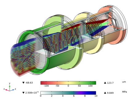
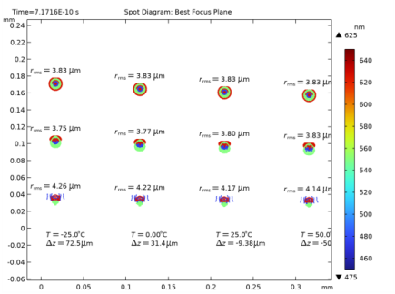
Locate the Annotation section. In the Text text field, type $T = eval(T0-0[degC])^\circ$C \\ $\Delta z = eval((162.79248823021723[mm]-aveop1(z))/1[um])\,\unicode{\mu}$m. The numerical value is the z-component of the Intersection Point 3D dataset for this plot.
|
|
6
|
|
7
|
|
8
|
|
9
|
|
1
|
|
2
|
|
3
|
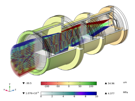
In the Text text field, type $T = eval(T0-0[degC])^\circ$C \\ $\Delta z = eval((162.78305987604173[mm]-aveop1(z))/1[um])\,\unicode{\mu}$m.
|
|
4
|
|
5
|
|
1
|
|
2
|
|
3
|
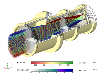
In the Text text field, type $T = eval(T0-0[degC])^\circ$C \\ $\Delta z = eval((162.7738443879646[mm]-aveop1(z))/1[um])\,\unicode{\mu}$m.
|
|
4
|
|
5
|
|
1
|
|
2
|
|
3
|
In the Text text field, type $T = eval(T0-0[degC])^\circ$C \\ $\Delta z = eval((162.76447789300707[mm]-aveop1(z))/1[um])\,\unicode{\mu}$m.
|
|
4
|
|
5
|
|
6
|