PDF

Lithium-Ion Battery Rate Capability
Introduction
A battery’s possible energy and power outputs are critical to consider when deciding in which type of device it can be used.
A cell with high rate capability is able to generate a considerable amount of power, as it suffers from little polarization (voltage loss) even at high current loads. In contrast, a low rate-capability cell has the opposite behavior. The former cell type is said to be power optimized, while the latter type is energy optimized.
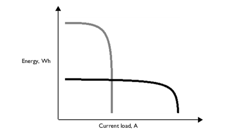
Characteristic for energy-optimized cells is that these have more capacity, and are thus able to supply more energy, but only for mild loads. Therefore, energy-optimized batteries are more suitable for portable electronics, for example, cell phones. The power energy-optimized ones fits, for example, power-demanding hybrid-electric vehicles better. The difference between these two types of cells is illustrated in Figure 1.
Figure 1: Comparison of energy outputs. Energy optimized cells (gray) can supply more energy but for lower current loads. Power optimized cells (black) work fine for higher current loads but can only provide a fraction of the energy.
This application performs a rate capability investigation of two lithium-ion battery cell designs using the Lithium-Ion Battery interface. You can also learn more about how to study rate capability with the Lithium-Ion Battery Internal Resistance application.
Model Definition
The model is set up for both MCMB/LMO and LTO/NMC battery cells. The materials are available from the Battery Material Library and mainly default settings are selected. The model domains consist of:
Cell 1) Graphite, MCMB (LixC6 graphite) active material and electronic conductor.
Cell 2) Lithium–titanate, LTO (Li4Ti5O12) active material and electronic conductor.
Cell 1) LMO (LiMn2O4 spinel) active material, electronic conductor, and filler.
Cell 2) NMC (LiNi1/3Mn1/3Co1/3O2) active material, electronic conductor, and filler.
Electrolyte: 1.0 M LiPF6 in EC:DEC (1:1 by weight)
The upper and lower cutoff voltages are set to 4.1 V and 3.3 V, respectively, for MCMB/LMO and 3.3 V and 0.5 V, respectively, for LTO/NMC. The cutoff voltages correspond to the potential difference between the open-circuit potentials of the positive and negative electrode active materials when the battery is either completely charged or fully discharged.
The Lithium-Ion Battery interface accounts for:
To investigate the rate capability, the battery is discharged from its fully charged state and charged from its fully discharge state. This is done for different current loads, defined in terms of C-rate with 1C being the current load to discharge a fully charged battery completely in 1 hour. This model bases the C-rate on the battery capacity, QB. For a 12 Ah battery 1C is thus equal to 12 A. The same definition is used in the Initial Cell Charge Distribution feature that is used in this model. It is also this feature that allows you to have initial cell state-of-charge (SOC) as a model input.
The energy and power outputs during the discharge are calculated and investigated in a Ragone plot. A Global ODEs and DAEs interface is used to calculate the energy output according to Equation 1.
(1)
The power output is computed by dividing the energy with the total discharge time.
An Event interface is also used to restrict the operation of the battery within the upper and lower cutoff voltages.
More battery parameters and additional variable definitions used here are found in the Lithium-Ion Battery Seed application.
Study settings
A parametric sweep where the current load is varied is included in the existing study.
Results and Discussion
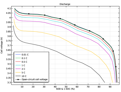
The current loads applied on the cell are 0.01C, 0.1C, 0.5C, 1C, 2C, 5C, and 10C. At discharge the initial cell voltage is set at the upper cutoff voltage, 4.1 V, and at charge to the lower cutoff voltage, 3.3 V, for the MCMB/LMO battery cell. In Figure 2, the cell voltage for the discharge loads is shown for the MCMB/LMO cell. A clear increase in polarization (voltage drop) with increased load is observed. Compared to the open-circuit voltage curve, the capacity utilization decreases considerably with increased load as well.
Figure 2: Cell voltage during 0.01C, 0.1C, 1C, 2C, 5C, and 10C discharge current load for the MCMB/LMO battery cell.
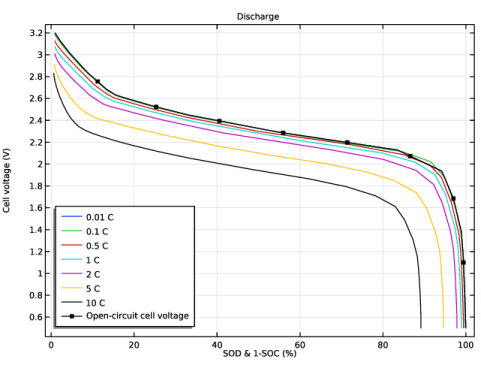
For the LTO/NMC battery cell, the initial cell voltage is set to the upper cutoff voltage, 3.2 V, at discharge and to the lower cutoff voltage, 0.5 V, at charge. In Figure 3, the cell voltage for the discharge loads is shown for the LTO/NMC cell. The observed increase in polarization with current load is slightly higher for this battery design. Less capacity is also discharged.
Figure 3: Cell voltage during 0.01C, 0.1C, 1C, 2C, 5C, and 10C discharge current load for the LTO/NMC battery cell.
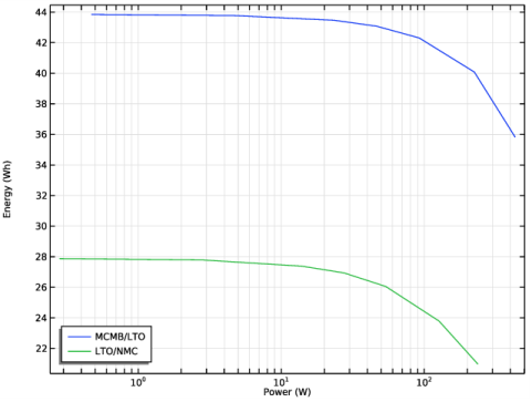
Figure 4 is a Ragone plot displaying both battery designs’ energy versus power output. The shape of the plot is characteristic for batteries. With increased energy output less power is obtained and vice versa. The shape of the Ragone plot can change drastically if the battery design is altered. A comparison of the MCMB/LMO and LTO/NMC data shows that the energy density is considerably lower in the LTO/NMC cell. This is mainly explained by the lower cell voltage of the cell (see Figure 2 and Figure 3). Improved rate capability would shift the slope further to the right along the x-axis, at the same time as the whole curve is shifted downward. The LTO/NMC cell has, despite the lower energy density, also worse rate capability. The rather small change in energy density with current load (~10%) for both cells indicates that both are rather power-optimized. To achieve better rate capability other design features than electrode chemistry can be changed, this is described in the Lithium-Ion Battery Internal Resistance application.
Figure 4: Ragone plot for the MCMB/LMO and LTO/NMC battery cells.
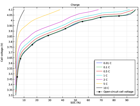
The charge behavior is normally harder to put into the context of rate capability. This is illustrated for the MCMB/LMO battery cell in Figure 5. The polarization is slightly more pronounced compared to discharge. However, most striking is that the charged capacity is considerably lower than the discharged capacity (less of SOC window is utilized). This mainly has to do with the shape of the open-circuit potential curves of the electrode active materials. The low capacity usage normally means that the active electrode material can handle peaks of medium-high current load, where the cell voltage exceeds that of a fully charged cell (>4.1 V), given that the voltage is within the stability window of the electrolyte.
Figure 5: Cell voltage during 0.01C, 0.1C, 1C, 2C, 5C, and 10C charge current load for the MCMB/LMO battery cell.
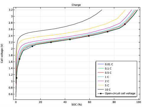
The cell voltage at charge load for the LTO/NMC cell is displayed in Figure 6. The charged capacity is also lower than the discharged capacity for this cell design, however, the polarization is in the same magnitude as for the discharge.
Figure 6: Cell voltage during 0.01C, 0.1C, 1C, 2C, 5C, and 10C charge current load for the LTO/NMC battery cell.
Application Library path: Battery_Design_Module/Batteries,_Lithium-Ion/li_battery_rate_capability
Modeling Instructions
Application Libraries
1
From the File menu, choose Application Libraries.
2
In the Application Libraries window, select Battery Design Module>Batteries, Lithium-Ion>li_battery_seed in the tree.
3
Global Definitions
Add parameters for controlling the C-rate as well as the upper and lower cutoff voltages for the battery cell.
Parameters 1
1
In the Model Builder window, under Global Definitions click Parameters 1.
2
In the Settings window for Parameters, locate the Parameters section.
3
Also modify the parameter value for Ecell_init as follows:
4
Definitions (comp1)
Load the variables from a text file.
Variables 1
1
In the Model Builder window, under Component 1 (comp1) right-click Definitions and choose Variables.
2
In the Settings window for Variables, locate the Variables section.
3
Click  Load from File.
4
Lithium-Ion Battery (liion)
Electrode Current -Current Load Rates
1
In the Model Builder window, under Component 1 (comp1)>Lithium-Ion Battery (liion) click Electrode Current 1.
2
In the Settings window for Electrode Current, type Electrode Current -Current Load Rates in the Label text field.
3
Locate the Electrode Current section. In the Is,total text field, type liion.I_1C*a.
Porous Electrode 1
In the Particle Intercalation nodes of the Porous Electrode features, it is useful to enable fast assembly in the particle dimension option. This option enables an alternative method for assembling of the diffusion equation in the particle dimension, that typically decreases computation time for 1D models. Note that the same diffusion equations are solved for regardless of assembly method. Additionally, specify the reference exchange current density for the electrode kinetics in the Porous Electrode Reaction nodes.
Particle Intercalation 1
1
In the Model Builder window, expand the Porous Electrode 1 node, then click Particle Intercalation 1.
2
In the Settings window for Particle Intercalation, click to expand the Particle Discretization section.
3
Select the Fast assembly in particle dimension check box.
Porous Electrode Reaction 1
1
In the Model Builder window, click Porous Electrode Reaction 1.
2
In the Settings window for Porous Electrode Reaction, locate the Electrode Kinetics section.
3
In the i0,ref(T) text field, type i0ref_neg.
Particle Intercalation 1
1
In the Model Builder window, expand the Porous Electrode 2 node, then click Particle Intercalation 1.
2
In the Settings window for Particle Intercalation, locate the Particle Discretization section.
3
Select the Fast assembly in particle dimension check box.
Porous Electrode Reaction 1
1
In the Model Builder window, click Porous Electrode Reaction 1.
2
In the Settings window for Porous Electrode Reaction, locate the Electrode Kinetics section.
3
In the i0,ref(T) text field, type i0ref_pos.
Component 1 (comp1)
For the rate capability investigation a Global equation that calculates the cumulative energy is set up.
Add Physics
1
In the Home toolbar, click  Add Physics to open the Add Physics window.
2
Go to the Add Physics window.
3
In the tree, select Mathematics>ODE and DAE Interfaces>Global ODEs and DAEs (ge).
4
Click Add to Component 1 in the window toolbar.
Cumulative Energy
In the Settings window for Global ODEs and DAEs, type Cumulative Energy in the Label text field.
Global Equations 1
1
In the Model Builder window, under Component 1 (comp1)>Cumulative Energy (ge) click Global Equations 1.
2
In the Settings window for Global Equations, locate the Global Equations section.
3
4
Locate the Units section. Click  Define Dependent Variable Unit.
5
In the Dependent variable quantity table, enter the following settings:
6
Click  Define Source Term Unit.
7
In the Source term quantity table, enter the following settings:
Component 1 (comp1)
Add an Events interface to control the cutoff voltages.
Add Physics
1
Go to the Add Physics window.
2
In the tree, select Mathematics>ODE and DAE Interfaces>Events (ev).
3
Click Add to Component 1 in the window toolbar.
4
In the Home toolbar, click  Add Physics to close the Add Physics window.
Events (ev)
Implicit Event 1
Define the cutoff at charge, STOP_CH.
1
Right-click Component 1 (comp1)>Events (ev) and choose Implicit Event.
2
In the Settings window for Implicit Event, locate the Event Conditions section.
3
In the Condition text field, type STOP_CH>0.
Implicit Event 2
Define the cutoff at discharge, STOP_DCH.
1
In the Physics toolbar, click  Global and choose Implicit Event.
2
In the Settings window for Implicit Event, locate the Event Conditions section.
3
In the Condition text field, type STOP_DCH>0.
Indicator States 1
Define the values of cell voltage, Ecell, for the cutoffs.
1
In the Physics toolbar, click  Global and choose Indicator States.
2
In the Settings window for Indicator States, locate the Indicator Variables section.
3
Study 1
Start by adding a Parametric sweep to the Study node.
In order to investigate several current loads, use a number of high initial voltages with discharge currents, and a number of low initial voltages with charge currents. Voltages and current loads are available in a text file.
Parametric Sweep
1
In the Study toolbar, click  Parametric Sweep.
2
In the Settings window for Parametric Sweep, locate the Study Settings section.
3
Click  Load from File.
4
Step 1: Current Distribution Initialization
Shut off the Events and Cumulative Energy Density interfaces in the first study step.
1
In the Model Builder window, click Step 1: Current Distribution Initialization.
2
In the Settings window for Current Distribution Initialization, locate the Physics and Variables Selection section.
3
In the table, clear the Solve for check boxes for Cumulative Energy (ge) and Events (ev).
Step 2: Time Dependent
Enter the times the model should be solved for in the Time Dependent (second) study step.
1
In the Model Builder window, click Step 2: Time Dependent.
2
In the Settings window for Time Dependent, locate the Study Settings section.
3
In the Output times text field, type 0 500000.
Solution 1 (sol1)
Select the following time-dependent settings to speed up the simulation and to save the solution.
1
In the Study toolbar, click  Show Default Solver.
Store the actual steps taken by the solver to make sure to capture any sudden steep voltage changes.
2
In the Model Builder window, expand the Solution 1 (sol1) node, then click Time-Dependent Solver 1.
3
In the Settings window for Time-Dependent Solver, locate the General section.
4
From the Times to store list, choose Steps taken by solver.
Store only every 3rd time step. This reduces the solution and resulting file size.
5
In the Store every Nth step text field, type 3.
6
Click to expand the Time Stepping section. Select the Initial step check box.
7
In the Event tolerance text field, type 1e-3.
8
Select the Nonlinear controller check box.
9
Click to expand the Output section. Right-click Study 1>Solver Configurations>Solution 1 (sol1)>Time-Dependent Solver 1 and choose Stop Condition.
Add a Stop Condition defined by the Events interface.
10
In the Settings window for Stop Condition, locate the Stop Events section.
11
In the table, select the Active check boxes for Events (ev)/Implicit Event 1 and Events (ev)/Implicit Event 2.
12
Locate the Output at Stop section. Clear the Add warning check box.
Mesh 1
1
In the Model Builder window, under Component 1 (comp1) click Mesh 1.
2
In the Settings window for Mesh, locate the Sequence Type section.
3
From the list, choose User-controlled mesh.
Size 1
1
In the Model Builder window, under Component 1 (comp1)>Mesh 1 click Size 1.
2
In the Settings window for Size, locate the Element Size section.
3
From the Predefined list, choose Extremely fine.
4
Click  Build All.
Study 1
1
In the Model Builder window, click Study 1.
2
In the Settings window for Study, locate the Study Settings section.
3
Clear the Generate default plots check box.
4
Clear the Generate convergence plots check box.
5
In the Study toolbar, click  Compute.
Parametric Solutions 1 (sol3)
In the Model Builder window, under Study 1>Solver Configurations right-click Parametric Solutions 1 (sol3) and choose Solution>Copy.
Copied Parametric Solutions MCMB/LMO
1
In the Model Builder window, under Study 1>Solver Configurations click Parametric Solutions 1 - Copy 1 (sol18).
2
In the Settings window for Solution, type Copied Parametric Solutions MCMB/LMO in the Label text field.
Results
Cell Voltages Discharge MCMB/LMO
1
In the Home toolbar, click  Add Plot Group and choose 1D Plot Group.
2
In the Settings window for 1D Plot Group, type Cell Voltages Discharge MCMB/LMO in the Label text field.
3
Locate the Data section. From the Dataset list, choose None.
4
Click to expand the Title section. From the Title type list, choose Manual.
5
In the Title text area, type Discharge.
6
Locate the Plot Settings section. Select the x-axis label check box.
7
8
Select the y-axis label check box.
9
10
Locate the Legend section. From the Position list, choose Lower left.
Global 1
1
Right-click Cell Voltages Discharge MCMB/LMO and choose Global.
2
In the Settings window for Global, locate the Data section.
3
From the Dataset list, choose Study 1/Copied Parametric Solutions MCMB/LMO (sol18).
4
From the Parameter selection (a) list, choose From list.
5
In the Parameter values (a (C)) list, choose -0.01, -0.1, -0.5, -1, -2, -5, and -10.
6
Click Replace Expression in the upper-right corner of the y-Axis Data section. From the menu, choose Component 1 (comp1)>Definitions>Variables>Ecell - Battery cell voltage - V.
7
Locate the x-Axis Data section. From the Axis source data list, choose Inner solutions.
8
From the Parameter list, choose Expression.
9
In the Expression text field, type (1-SOCcell)*100.
10
Click to expand the Legends section. From the Legends list, choose Evaluated.
11
In the Legend text field, type eval(-a) C.
Global 2
1
In the Model Builder window, right-click Cell Voltages Discharge MCMB/LMO and choose Global.
2
In the Settings window for Global, locate the Data section.
3
From the Dataset list, choose Study 1/Copied Parametric Solutions MCMB/LMO (sol18).
4
From the Parameter selection (a) list, choose First.
5
Click Replace Expression in the upper-right corner of the y-Axis Data section. From the menu, choose Component 1 (comp1)>Definitions>Variables>EOCVcell - Open-circuit cell voltage, coulombic - V.
6
Locate the x-Axis Data section. From the Axis source data list, choose Inner solutions.
7
From the Parameter list, choose Expression.
8
In the Expression text field, type (1-SOCcell)*100.
9
Click to expand the Coloring and Style section. From the Color list, choose Black.
10
Find the Line markers subsection. From the Marker list, choose Point.
11
Locate the Legends section. From the Legends list, choose Manual.
12
13
In the Cell Voltages Discharge MCMB/LMO toolbar, click  Plot.
Global Evaluation 2
Create a Ragone plot as follows:
1
In the Results toolbar, click  Global Evaluation.
2
In the Settings window for Global Evaluation, locate the Data section.
3
From the Dataset list, choose Study 1/Parametric Solutions 1 (sol3).
4
From the Parameter selection (a) list, choose Manual.
5
In the Parameter indices (1-14) text field, type range(1,1,7).
6
From the Time selection list, choose Last.
7
Locate the Expressions section. In the table, enter the following settings:
8
Clicknext to  Evaluate, then choose New Table.
Ragone Plot
1
In the Results toolbar, click  1D Plot Group.
2
In the Settings window for 1D Plot Group, type Ragone Plot in the Label text field.
3
Locate the Title section. From the Title type list, choose None.
4
Locate the Plot Settings section. Select the x-axis label check box.
5
6
Select the y-axis label check box.
7
8
Locate the Axis section. Select the x-axis log scale check box.
Table Graph 1
1
Right-click Ragone Plot and choose Table Graph.
2
In the Settings window for Table Graph, locate the Data section.
3
From the Table list, choose Table 2.
4
From the x-axis data list, choose Power (W).
5
From the Plot columns list, choose Manual.
6
In the Columns list, select Energy (W*h).
7
Click to expand the Legends section. Select the Show legends check box.
8
From the Legends list, choose Manual.
9
10
In the Ragone Plot toolbar, click  Plot.
Global Definitions
Benchmark the MCMB/LMO cell against a LTO/NMC cell.
Add the two materials from the Battery Material Library.
Add Material
1
In the Home toolbar, click  Add Material to open the Add Material window.
2
Go to the Add Material window.
3
In the tree, select Battery>Electrodes>LTO, Li4Ti5O12 (Negative, Li-ion Battery).
4
Click the right end of the Add to Component split button in the window toolbar.
5
From the menu, choose Add to Global Materials.
6
In the tree, select Battery>Electrodes>NMC 111, LiNi0.33Mn0.33Co0.33O2 (Positive, Li-ion Battery).
7
Click the right end of the Add to Component split button in the window toolbar.
8
From the menu, choose Add to Global Materials.
9
In the Home toolbar, click  Add Material to close the Add Material window.
Materials
Material Link 2 (matlnk2)
1
In the Model Builder window, expand the Component 1 (comp1)>Materials node, then click Material Link 2 (matlnk2).
2
In the Settings window for Material Link, locate the Link Settings section.
3
From the Material list, choose LTO, Li4Ti5O12 (Negative, Li-ion Battery) (mat4).
Material Link 3 (matlnk3)
1
In the Model Builder window, click Material Link 3 (matlnk3).
2
In the Settings window for Material Link, locate the Link Settings section.
3
From the Material list, choose NMC 111, LiNi0.33Mn0.33Co0.33O2 (Positive, Li-ion Battery) (mat5).
Global Definitions
Adjust the upper and lower cutoff voltages to the new chemistry.
Parameters 1
1
In the Model Builder window, under Global Definitions click Parameters 1.
2
In the Settings window for Parameters, locate the Parameters section.
3
Lithium-Ion Battery (liion)
Initial Cell Charge Distribution 1
The negative LTO electrode material does not cause as pronounced SEI layer formation. This means that the cyclable lithium loss at assemble and excess negative electrode material can both be set to zero.
1
In the Model Builder window, under Component 1 (comp1)>Lithium-Ion Battery (liion) click Initial Cell Charge Distribution 1.
2
In the Settings window for Initial Cell Charge Distribution, locate the Battery Cell Electrode Balancing section.
3
In the fhost,neg,ex text field, type 0.
4
In the fcycl,loss text field, type 0.
Study 1
In the Home toolbar, click  Compute.
Results
Cell Voltages Discharge LTO/NMC
1
In the Model Builder window, right-click Cell Voltages Discharge MCMB/LMO and choose Duplicate.
2
In the Settings window for 1D Plot Group, type Cell Voltages Discharge LTO/NMC in the Label text field.
Global 1
1
In the Model Builder window, expand the Cell Voltages Discharge LTO/NMC node, then click Global 1.
2
In the Settings window for Global, locate the Data section.
3
From the Dataset list, choose Study 1/Parametric Solutions 1 (sol3).
Global 2
1
In the Model Builder window, click Global 2.
2
In the Settings window for Global, locate the Data section.
3
From the Dataset list, choose Study 1/Parametric Solutions 1 (sol3).
4
In the Cell Voltages Discharge LTO/NMC toolbar, click  Plot.
Global Evaluation 2
Update the Ragone plot as follows:
In the Model Builder window, under Results>Derived Values right-click Global Evaluation 2 and choose Evaluate>New Table.
Table Graph 2
1
In the Model Builder window, under Results>Ragone Plot right-click Table Graph 1 and choose Duplicate.
2
In the Settings window for Table Graph, locate the Data section.
3
From the Table list, choose Table 3.
4
Locate the Legends section. In the table, enter the following settings:
5
In the Ragone Plot toolbar, click  Plot.
Ragone Plot
1
In the Model Builder window, click Ragone Plot.
2
In the Settings window for 1D Plot Group, locate the Legend section.
3
From the Position list, choose Lower left.
4
In the Ragone Plot toolbar, click  Plot.
Cell Voltages Charge MCMB/LMO
1
In the Model Builder window, right-click Cell Voltages Discharge MCMB/LMO and choose Duplicate.
2
In the Settings window for 1D Plot Group, type Cell Voltages Charge MCMB/LMO in the Label text field.
3
Locate the Title section. In the Title text area, type Charge.
4
Locate the Plot Settings section. In the x-axis label text field, type SOC (%).
Global 1
1
In the Model Builder window, expand the Cell Voltages Charge MCMB/LMO node, then click Global 1.
2
In the Settings window for Global, locate the Data section.
3
In the Parameter values (a (C)) list, choose 0.01, 0.1, 0.5, 1, 2, 5, and 10.
4
Locate the x-Axis Data section. In the Expression text field, type SOCcell*100.
5
Locate the Legends section. In the Legend text field, type eval(a) C.
Global 2
1
In the Model Builder window, click Global 2.
2
In the Settings window for Global, locate the x-Axis Data section.
3
In the Expression text field, type SOCcell*100.
Cell Voltages Charge MCMB/LMO
1
In the Model Builder window, click Cell Voltages Charge MCMB/LMO.
2
In the Settings window for 1D Plot Group, locate the Legend section.
3
From the Position list, choose Lower right.
4
In the Cell Voltages Charge MCMB/LMO toolbar, click  Plot.
Cell Voltages Charge LTO/NMC
1
Right-click Cell Voltages Charge MCMB/LMO and choose Duplicate.
2
In the Settings window for 1D Plot Group, type Cell Voltages Charge LTO/NMC in the Label text field.
Global 1
1
In the Model Builder window, expand the Cell Voltages Charge LTO/NMC node, then click Global 1.
2
In the Settings window for Global, locate the Data section.
3
From the Dataset list, choose Study 1/Parametric Solutions 1 (sol3).
Global 2
1
In the Model Builder window, click Global 2.
2
In the Settings window for Global, locate the Data section.
3
From the Dataset list, choose Study 1/Parametric Solutions 1 (sol3).
4
In the Cell Voltages Charge LTO/NMC toolbar, click  Plot.