|
|
|


|
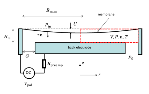
18 μm
|
||
|
54 μm
|
||
|
7 μm
|
||
|
νm
|


|
1
|
|
2
|
|
3
|
Click Add.
|
|
4
|
|
5
|
Click Add.
|
|
6
|
In the Select Physics tree, select Acoustics>Thermoviscous Acoustics>Thermoviscous Acoustics, Frequency Domain (ta).
|
|
7
|
Click Add.
|
|
8
|
|
9
|
Click Add.
|
|
10
|
|
11
|
In the Displacement field components table, enter the following settings:
|
|
12
|
Click
|
|
13
|
In the Select Study tree, select Preset Studies for Selected Physics Interfaces>Membrane>Frequency Domain, Prestressed.
|
|
14
|
Click
|
|
1
|
|
2
|
|
3
|
|
4
|
Browse to the model’s Application Libraries folder and double-click the file condenser_microphone_parameters.txt.
|
|
1
|
|
2
|
|
3
|
|
1
|
|
2
|
|
3
|
|
4
|
|
5
|
|
1
|
|
2
|
|
3
|
|
4
|
|
5
|
|
6
|
|
1
|
|
2
|
|
3
|
|
5
|
|
1
|
|
2
|
|
3
|
|
4
|
Browse to the model’s Application Libraries folder and double-click the file condenser_microphone_variables.txt.
|
|
1
|
|
2
|
|
3
|
|
1
|
|
2
|
|
3
|
In the tree, select Built-in>Air.
|
|
4
|
|
5
|
|
1
|
In the Model Builder window, under Component 1 (comp1) right-click Electrostatics (es) and choose the boundary condition Terminal.
|
|
3
|
|
4
|
|
1
|
|
2
|
|
3
|
|
1
|
|
2
|
|
3
|
|
1
|
|
2
|
|
4
|
|
1
|
|
2
|
|
4
|
|
1
|
|
2
|
|
4
|
|
1
|
|
3
|
|
4
|
|
1
|
In the Physics toolbar, click
|
|
2
|
In the Settings window for Thermoviscous Acoustic-Structure Boundary, locate the Boundary Selection section.
|
|
3
|
|
1
|
|
2
|
|
3
|
|
1
|
In the Model Builder window, under Component 1 (comp1)>Membrane (mbrn) click Thickness and Offset 1.
|
|
2
|
|
3
|
|
1
|
|
2
|
|
3
|
|
4
|
|
5
|
|
1
|
|
2
|
|
3
|
|
1
|
|
1
|
|
2
|
|
3
|
|
4
|
|
1
|
|
2
|
|
3
|
|
4
|
|
5
|
|
1
|
|
2
|
|
3
|
|
1
|
|
1
|
|
1
|
|
2
|
|
3
|
|
4
|
Click in the Graphics window and then press Ctrl+A to select both domains.
|
|
5
|
|
1
|
|
3
|
|
4
|
|
1
|
|
3
|
|
4
|
|
5
|
|
6
|
|
7
|
|
1
|
|
3
|
|
4
|
|
1
|
|
2
|
|
3
|
|
1
|
|
3
|
|
4
|
|
5
|
|
6
|
|
7
|
|
1
|
|
2
|
|
3
|
|
1
|
|
2
|
|
3
|
|
4
|
|
5
|
|
1
|
|
2
|
|
3
|
|
4
|
|
5
|
Locate the Expressions section. In the table, enter the following settings:
|
|
6
|
|
7
|
Click
|
|
1
|
Go to the Table window.
|
|
1
|
|
2
|
|
1
|
|
2
|
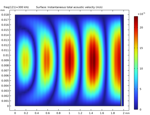
In the Settings window for Surface, click Replace Expression in the upper-right corner of the Expression section. From the menu, choose Component 1 (comp1)>Thermoviscous Acoustics, Frequency Domain>Acceleration and velocity>ta.v_inst - Instantaneous total acoustic velocity - m/s.
|
|
3
|
|
1
|
|
2
|
|
3
|
|
4
|
Click
|
|
5
|
|
1
|
|
2
|
|
1
|
|
1
|
|
2
|
|
3
|
|
4
|
|
5
|
|
6
|
|
1
|
|
2
|
|
3
|
|
4
|
|
5
|
|
6
|
|
7
|
|
1
|
|
2
|
|
3
|
|
1
|
|
2
|
|
3
|
|
4
|
|
5
|
|
6
|
|
7
|
|
1
|
|
2
|
|
3
|
|
1
|
|
2
|
|
3
|
|
4
|
|
1
|
|
2
|
|
3
|
|
4
|
|
5
|
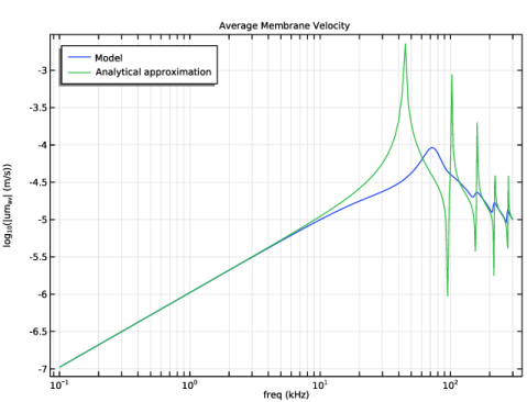
Select the y-axis label check box. In the associated text field, type log<sub>10</sub>(|um<sub>av</sub>| (m/s)).
|
|
6
|
|
1
|
|
2
|
|
4
|
|
5
|
|
1
|
|
2
|
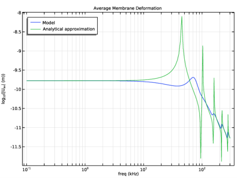
In the Settings window for 1D Plot Group, type Average Membrane Deformation in the Label text field.
|
|
3
|
|
4
|
|
5
|
Select the y-axis label check box. In the associated text field, type log<sub>10</sub>(|U<sub>av</sub>| (m)).
|
|
6
|
|
1
|
|
2
|
|
4
|
|
5
|
|
1
|
|
2
|
|
1
|
|
2
|
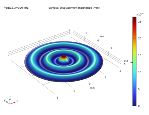
In the Settings window for Surface, click Replace Expression in the upper-right corner of the Expression section. From the menu, choose Component 1 (comp1)>Membrane>Displacement>mbrn.disp - Displacement magnitude - m.
|
|
1
|
|
2
|
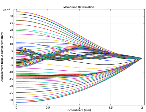
In the Settings window for Deformation, click Replace Expression in the upper-right corner of the Expression section. From the menu, choose Component 1 (comp1)>Membrane>Displacement>um,vm,wm - Displacement field.
|
|
3
|