|
|
|
|
1
|
|
2
|
|
3
|
Click Add.
|
|
4
|
Click
|
|
5
|
|
6
|
Click
|
|
1
|
|
2
|
Browse to the model’s Application Libraries folder and double-click the file chamber_music_hall_geom_sequence.mph.
|
|
3
|
|
1
|
|
2
|
|
3
|
|
4
|
Browse to the model’s Application Libraries folder and double-click the file chamber_music_hall_parameters1.txt.
|
|
1
|
|
2
|
In the Settings window for Parameters, type Parameters 2 - Source and receiver positions in the Label text field.
|
|
3
|
|
4
|
Browse to the model’s Application Libraries folder and double-click the file chamber_music_hall_parameters2.txt.
|
|
1
|
|
2
|
|
3
|
|
4
|
Click
|
|
5
|
Browse to the model’s Application Libraries folder and double-click the file chamber_music_hall_air_attenuation.txt.
|
|
6
|
Click
|
|
7
|
|
8
|
Find the Functions subsection. In the table, enter the following settings:
|
|
9
|
Locate the Interpolation and Extrapolation section. From the Interpolation list, choose Nearest neighbor.
|
|
10
|
|
11
|
In the Argument table, enter the following settings:
|
|
12
|
|
1
|
|
2
|
|
3
|
|
4
|
Click
|
|
5
|
Browse to the model’s Application Libraries folder and double-click the file chamber_music_hall_ceiling.csv.
|
|
6
|
|
7
|
Find the Functions subsection. In the table, enter the following settings:
|
|
8
|
Locate the Interpolation and Extrapolation section. From the Interpolation list, choose Nearest neighbor.
|
|
9
|
|
10
|
In the Argument table, enter the following settings:
|
|
11
|
|
1
|
|
2
|
|
3
|
|
4
|
Click
|
|
5
|
Browse to the model’s Application Libraries folder and double-click the file chamber_music_hall_floor.csv.
|
|
6
|
|
7
|
Find the Functions subsection. In the table, enter the following settings:
|
|
8
|
Locate the Interpolation and Extrapolation section. From the Interpolation list, choose Nearest neighbor.
|
|
9
|
|
10
|
In the Argument table, enter the following settings:
|
|
11
|
|
1
|
|
2
|
|
3
|
|
4
|
Click
|
|
5
|
Browse to the model’s Application Libraries folder and double-click the file chamber_music_hall_plaster.csv.
|
|
6
|
|
7
|
Find the Functions subsection. In the table, enter the following settings:
|
|
8
|
Locate the Interpolation and Extrapolation section. From the Interpolation list, choose Nearest neighbor.
|
|
9
|
|
10
|
In the Argument table, enter the following settings:
|
|
11
|
|
1
|
|
2
|
|
3
|
|
4
|
Click
|
|
5
|
Browse to the model’s Application Libraries folder and double-click the file chamber_music_hall_seating.csv.
|
|
6
|
|
7
|
Find the Functions subsection. In the table, enter the following settings:
|
|
8
|
Locate the Interpolation and Extrapolation section. From the Interpolation list, choose Nearest neighbor.
|
|
9
|
|
10
|
In the Argument table, enter the following settings:
|
|
11
|
|
1
|
|
2
|
|
3
|
|
4
|
Click
|
|
5
|
Browse to the model’s Application Libraries folder and double-click the file chamber_music_hall_stagepanels.csv.
|
|
6
|
|
7
|
Find the Functions subsection. In the table, enter the following settings:
|
|
8
|
Locate the Interpolation and Extrapolation section. From the Interpolation list, choose Nearest neighbor.
|
|
9
|
|
10
|
In the Argument table, enter the following settings:
|
|
11
|
|
1
|
|
2
|
|
3
|
|
4
|
Click
|
|
5
|
Browse to the model’s Application Libraries folder and double-click the file chamber_music_hall_structuredplaster.csv.
|
|
6
|
|
7
|
Find the Functions subsection. In the table, enter the following settings:
|
|
8
|
Locate the Interpolation and Extrapolation section. From the Interpolation list, choose Nearest neighbor.
|
|
9
|
|
10
|
In the Argument table, enter the following settings:
|
|
11
|
|
1
|
|
2
|
|
3
|
|
4
|
Click
|
|
5
|
Browse to the model’s Application Libraries folder and double-click the file chamber_music_hall_windows.csv.
|
|
6
|
|
7
|
Find the Functions subsection. In the table, enter the following settings:
|
|
8
|
Locate the Interpolation and Extrapolation section. From the Interpolation list, choose Nearest neighbor.
|
|
9
|
|
10
|
In the Argument table, enter the following settings:
|
|
11
|
|
1
|
|
2
|
|
3
|
|
4
|
Click
|
|
5
|
Browse to the model’s Application Libraries folder and double-click the file chamber_music_hall_EDT.txt.
|
|
6
|
|
7
|
Find the Functions subsection. In the table, enter the following settings:
|
|
8
|
Locate the Interpolation and Extrapolation section. From the Interpolation list, choose Nearest neighbor.
|
|
9
|
|
10
|
In the Argument table, enter the following settings:
|
|
11
|
|
1
|
|
2
|
|
3
|
|
4
|
Click
|
|
5
|
Browse to the model’s Application Libraries folder and double-click the file chamber_music_hall_T20.txt.
|
|
6
|
|
7
|
Find the Functions subsection. In the table, enter the following settings:
|
|
8
|
Locate the Interpolation and Extrapolation section. From the Interpolation list, choose Nearest neighbor.
|
|
9
|
|
10
|
In the Argument table, enter the following settings:
|
|
11
|
|
1
|
|
2
|
|
3
|
|
4
|
Click
|
|
5
|
Browse to the model’s Application Libraries folder and double-click the file chamber_music_hall_C80.txt.
|
|
6
|
|
7
|
Find the Functions subsection. In the table, enter the following settings:
|
|
8
|
Locate the Interpolation and Extrapolation section. From the Interpolation list, choose Nearest neighbor.
|
|
9
|
|
10
|
In the Argument table, enter the following settings:
|
|
11
|
|
1
|
|
2
|
|
3
|
|
4
|
Click
|
|
5
|
Browse to the model’s Application Libraries folder and double-click the file chamber_music_hall_D50.txt.
|
|
6
|
|
7
|
Find the Functions subsection. In the table, enter the following settings:
|
|
8
|
Locate the Interpolation and Extrapolation section. From the Interpolation list, choose Nearest neighbor.
|
|
9
|
|
10
|
In the Argument table, enter the following settings:
|
|
11
|
|
1
|
|
2
|
|
3
|
|
4
|
Locate the Material Properties of Exterior and Unmeshed Domains section. In the cext text field, type c0.
|
|
5
|
|
6
|
|
7
|
|
1
|
|
2
|
|
3
|
|
1
|
|
2
|
|
3
|
|
4
|
Locate the Wall Condition section. From the Wall condition list, choose Mixed diffuse and specular reflection.
|
|
5
|
|
6
|
|
7
|
|
1
|
|
2
|
|
3
|
|
4
|
Locate the Wall Condition section. From the Wall condition list, choose Mixed diffuse and specular reflection.
|
|
5
|
|
6
|
|
7
|
|
1
|
|
2
|
|
3
|
|
4
|
Locate the Wall Condition section. From the Wall condition list, choose Mixed diffuse and specular reflection.
|
|
5
|
|
6
|
|
7
|
|
1
|
|
2
|
|
3
|
|
4
|
Locate the Wall Condition section. From the Wall condition list, choose Mixed diffuse and specular reflection.
|
|
5
|
|
6
|
|
7
|
|
1
|
|
2
|
|
3
|
|
4
|
Locate the Wall Condition section. From the Wall condition list, choose Mixed diffuse and specular reflection.
|
|
5
|
|
6
|
|
7
|
|
1
|
|
2
|
|
3
|
|
4
|
Locate the Wall Condition section. From the Wall condition list, choose Mixed diffuse and specular reflection.
|
|
5
|
|
6
|
|
7
|
|
1
|
|
2
|
|
3
|
|
4
|
Locate the Wall Condition section. From the Wall condition list, choose Mixed diffuse and specular reflection.
|
|
5
|
|
6
|
Locate the Reflection Coefficients Model section. In the αs text field, type a_structuredplaster(f0).
|
|
7
|
|
1
|
|
2
|
In the Settings window for Release from Grid, type Release from Grid - Source 1 in the Label text field.
|
|
3
|
|
4
|
|
5
|
|
6
|
|
7
|
|
8
|
|
1
|
|
2
|
In the Settings window for Release from Grid, type Release from Grid - Source 2 in the Label text field.
|
|
3
|
|
4
|
|
5
|
|
6
|
|
7
|
|
8
|
|
1
|
|
2
|
|
3
|
|
4
|
|
5
|
|
1
|
|
2
|
|
3
|
|
1
|
|
2
|
|
3
|
|
4
|
|
1
|
|
2
|
|
3
|
|
4
|
|
1
|
|
2
|
|
3
|
Click
|
|
6
|
Click
|
|
7
|
|
8
|
|
9
|
|
10
|
|
11
|
Click Replace.
|
|
1
|
|
2
|
|
3
|
|
4
|
|
5
|
Locate the Physics and Variables Selection section. Select the Modify model configuration for study step check box.
|
|
6
|
|
7
|
Right-click and choose Disable.
|
|
1
|
|
2
|
|
3
|
Find the Studies subsection. In the Select Study tree, select Preset Studies for Selected Physics Interfaces>Ray Tracing.
|
|
4
|
|
5
|
|
1
|
|
2
|
|
1
|
|
2
|
|
3
|
Click
|
|
6
|
Click
|
|
7
|
|
8
|
|
9
|
|
10
|
|
11
|
Click Replace.
|
|
1
|
|
2
|
|
3
|
|
4
|
|
5
|
Locate the Physics and Variables Selection section. Select the Modify model configuration for study step check box.
|
|
6
|
|
7
|
Click
|
|
1
|
|
2
|
|
3
|
|
4
|
|
5
|
|
6
|
|
7
|
|
8
|
Click the Save tab.
|
|
9
|
|
10
|
Click OK.
|
|
1
|
|
2
|
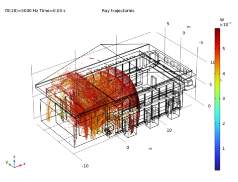
In the Settings window for 3D Plot Group, type Ray Trajectories (rac) - Source 1 in the Label text field.
|
|
3
|
|
4
|
|
1
|
In the Model Builder window, expand the Ray Trajectories (rac) - Source 1 node, then click Ray Trajectories 1.
|
|
2
|
|
3
|
|
4
|
|
1
|
|
2
|
|
3
|
|
4
|
|
1
|
|
2
|
|
3
|
|
4
|
|
5
|
|
6
|
|
7
|
|
8
|
|
9
|
|
10
|
|
1
|
|
2
|
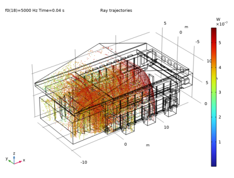
In the Settings window for 3D Plot Group, type Ray Trajectories (rac) - Source 2 in the Label text field.
|
|
3
|
|
4
|
|
1
|
In the Model Builder window, expand the Ray Trajectories (rac) - Source 2 node, then click Ray Trajectories 1.
|
|
2
|
|
3
|
|
4
|
|
1
|
|
2
|
|
3
|
|
4
|
|
1
|
|
2
|
|
3
|
|
4
|
|
5
|
|
6
|
|
7
|
|
1
|
|
2
|
|
3
|
|
4
|
|
5
|
|
6
|
|
7
|
|
1
|
|
2
|
|
3
|
|
4
|
|
5
|
|
6
|
|
7
|
|
1
|
|
2
|
|
3
|
|
4
|
|
5
|
|
6
|
|
7
|
|
1
|
|
2
|
|
3
|
|
4
|
|
5
|
|
6
|
|
7
|
|
1
|
|
2
|
|
3
|
|
4
|
|
5
|
|
6
|
|
7
|
|
8
|
|
1
|
|
2
|
|
3
|
|
4
|
|
5
|
|
6
|
|
7
|
|
8
|
|
1
|
|
2
|
|
3
|
|
4
|
|
5
|
|
6
|
|
7
|
|
8
|
|
1
|
|
2
|
|
3
|
|
4
|
|
5
|
|
6
|
|
7
|
|
8
|
|
1
|
|
2
|
|
3
|
|
4
|
|
5
|
|
6
|
|
7
|
|
8
|
|
1
|
|
2
|
|
3
|
|
4
|
|
1
|
|
2
|
|
3
|
|
4
|
|
1
|
|
2
|
|
3
|
|
4
|
|
5
|
|
6
|
|
7
|
|
8
|
|
9
|
|
10
|
|
11
|
|
12
|
|
13
|
|
14
|
|
1
|
|
2
|
|
3
|
|
4
|
|
1
|
|
2
|
|
3
|
|
4
|
|
1
|
|
2
|
|
3
|
|
4
|
|
5
|
|
6
|
|
7
|
|
8
|
|
9
|
|
10
|
|
11
|
|
12
|
|
13
|
|
14
|
|
1
|
|
2
|
|
3
|
|
4
|
|
1
|
|
2
|
|
3
|
|
4
|
|
1
|
|
2
|
|
3
|
|
4
|
|
5
|
|
6
|
|
7
|
|
8
|
|
9
|
|
10
|
|
11
|
|
12
|
|
13
|
|
14
|
|
1
|
|
2
|
|
3
|
|
4
|
|
1
|
|
2
|
|
3
|
|
4
|
|
1
|
|
2
|
|
3
|
|
4
|
|
5
|
|
6
|
|
7
|
|
8
|
|
9
|
|
10
|
|
11
|
|
12
|
|
13
|
|
14
|
|
1
|
|
2
|
|
3
|
|
4
|
|
1
|
|
2
|
|
3
|
|
4
|
|
1
|
|
2
|
|
3
|
|
4
|
|
5
|
|
6
|
|
7
|
|
8
|
|
9
|
|
10
|
|
11
|
|
12
|
|
13
|
|
14
|
|
1
|
|
2
|
|
3
|
|
4
|
|
1
|
|
2
|
|
3
|
|
4
|
|
1
|
|
2
|
|
3
|
|
4
|
|
5
|
|
6
|
|
7
|
|
8
|
|
9
|
|
10
|
|
11
|
|
12
|
|
13
|
|
14
|
|
1
|
|
2
|
|
3
|
|
4
|
|
1
|
|
2
|
|
3
|
|
4
|
|
1
|
|
2
|
|
3
|
|
4
|
|
5
|
|
6
|
|
7
|
|
8
|
|
9
|
|
10
|
|
11
|
|
12
|
|
13
|
|
14
|
|
1
|
|
2
|
|
3
|
|
4
|
|
1
|
|
2
|
|
3
|
|
4
|
|
1
|
|
2
|
|
3
|
|
4
|
|
5
|
|
6
|
|
7
|
|
8
|
|
9
|
|
10
|
|
11
|
|
12
|
|
13
|
|
14
|
|
1
|
|
2
|
|
3
|
|
4
|
|
1
|
|
2
|
|
3
|
|
4
|
|
1
|
|
2
|
|
3
|
|
4
|
|
5
|
|
6
|
|
7
|
|
8
|
|
9
|
|
10
|
|
11
|
|
12
|
|
13
|
|
14
|
|
1
|
|
2
|
|
3
|
|
4
|
|
1
|
|
2
|
|
3
|
|
4
|
|
1
|
|
2
|
|
3
|
|
4
|
|
5
|
|
6
|
|
7
|
|
8
|
|
9
|
|
10
|
|
11
|
|
12
|
|
13
|
|
14
|
|
1
|
In the Model Builder window, under Results, Ctrl-click to select Impulse response 1_1, Impulse response 1_2, Impulse response 1_3, Impulse response 1_4, Impulse response 1_5, Impulse response 2_1, Impulse response 2_2, Impulse response 2_3, Impulse response 2_4, and Impulse response 2_5.
|
|
2
|
Right-click and choose Group.
|
|
1
|
|
2
|
|
1
|
|
2
|
|
1
|
|
2
|
|
1
|
|
2
|
|
1
|
|
2
|
|
1
|
|
2
|
|
1
|
|
2
|
|
1
|
|
2
|
|
1
|
|
2
|
|
1
|
|
2
|
|
1
|
|
2
|
|
3
|
|
4
|
Find the Functions subsection. In the table, enter the following settings:
|
|
5
|
Locate the Interpolation and Extrapolation section. From the Interpolation list, choose Nearest neighbor.
|
|
6
|
|
7
|
In the Argument table, enter the following settings:
|
|
1
|
|
2
|
|
3
|
|
4
|
|
5
|
Find the Functions subsection. In the table, enter the following settings:
|
|
6
|
Locate the Interpolation and Extrapolation section. From the Interpolation list, choose Nearest neighbor.
|
|
7
|
|
8
|
In the Argument table, enter the following settings:
|
|
1
|
|
2
|
|
3
|
|
4
|
|
5
|
Find the Functions subsection. In the table, enter the following settings:
|
|
6
|
Locate the Interpolation and Extrapolation section. From the Interpolation list, choose Nearest neighbor.
|
|
7
|
|
8
|
In the Argument table, enter the following settings:
|
|
1
|
|
2
|
|
3
|
|
4
|
|
5
|
Find the Functions subsection. In the table, enter the following settings:
|
|
6
|
Locate the Interpolation and Extrapolation section. From the Interpolation list, choose Nearest neighbor.
|
|
7
|
|
8
|
In the Argument table, enter the following settings:
|
|
1
|
|
2
|
|
3
|
|
4
|
|
5
|
Find the Functions subsection. In the table, enter the following settings:
|
|
6
|
Locate the Interpolation and Extrapolation section. From the Interpolation list, choose Nearest neighbor.
|
|
7
|
|
8
|
In the Argument table, enter the following settings:
|
|
1
|
|
2
|
|
3
|
|
4
|
|
5
|
Find the Functions subsection. In the table, enter the following settings:
|
|
6
|
Locate the Interpolation and Extrapolation section. From the Interpolation list, choose Nearest neighbor.
|
|
7
|
|
8
|
In the Argument table, enter the following settings:
|
|
1
|
|
2
|
|
3
|
|
4
|
|
5
|
Find the Functions subsection. In the table, enter the following settings:
|
|
6
|
Locate the Interpolation and Extrapolation section. From the Interpolation list, choose Nearest neighbor.
|
|
7
|
|
8
|
In the Argument table, enter the following settings:
|
|
1
|
|
2
|
|
3
|
|
4
|
|
5
|
Find the Functions subsection. In the table, enter the following settings:
|
|
6
|
Locate the Interpolation and Extrapolation section. From the Interpolation list, choose Nearest neighbor.
|
|
7
|
|
8
|
In the Argument table, enter the following settings:
|
|
1
|
|
2
|
|
3
|
|
4
|
|
5
|
Find the Functions subsection. In the table, enter the following settings:
|
|
6
|
Locate the Interpolation and Extrapolation section. From the Interpolation list, choose Nearest neighbor.
|
|
7
|
|
8
|
In the Argument table, enter the following settings:
|
|
1
|
|
2
|
|
3
|
|
4
|
|
5
|
Find the Functions subsection. In the table, enter the following settings:
|
|
6
|
Locate the Interpolation and Extrapolation section. From the Interpolation list, choose Nearest neighbor.
|
|
7
|
|
8
|
In the Argument table, enter the following settings:
|
|
1
|
|
2
|
|
3
|
|
4
|
|
5
|
|
1
|
|
2
|
|
1
|
|
2
|
|
3
|
Click
|
|
6
|
Click
|
|
7
|
|
8
|
|
9
|
|
10
|
|
11
|
Click Replace.
|
|
12
|
|
1
|
|
2
|
|
3
|
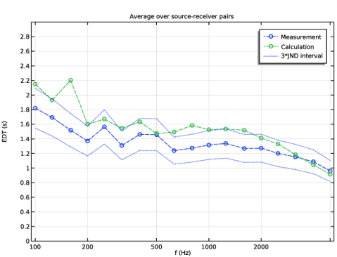
Locate the Data section. From the Dataset list, choose Study 3 - Empty for postprocessing/Parametric Solutions 3 (sol42).
|
|
4
|
|
5
|
|
6
|
|
7
|
|
8
|
|
9
|
|
10
|
In the associated text field, type EDT (s).
|
|
11
|
|
12
|
|
13
|
|
14
|
|
15
|
|
16
|
|
1
|
|
2
|
|
4
|
|
5
|
Click to expand the Coloring and Style section. Find the Line style subsection. From the Line list, choose Dashed.
|
|
6
|
|
7
|
|
8
|
|
1
|
|
2
|
|
4
|
|
5
|
Locate the Coloring and Style section. Find the Line style subsection. From the Line list, choose Dotted.
|
|
6
|
|
7
|
|
1
|
|
2
|
|
4
|
|
5
|
Locate the Coloring and Style section. Find the Line style subsection. From the Line list, choose Dotted.
|
|
6
|
|
7
|
|
8
|
|
1
|
|
2
|
|
3
|
Locate the Data section. From the Dataset list, choose Study 3 - Empty for postprocessing/Parametric Solutions 3 (sol42).
|
|
4
|
|
5
|
|
6
|
|
7
|
|
8
|
|
9
|
|
10
|
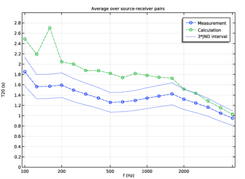
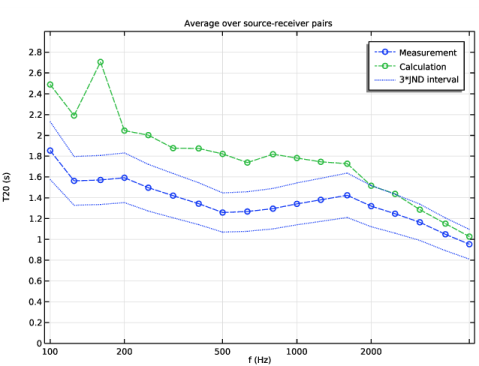
In the associated text field, type T20 (s).
|
|
11
|
|
12
|
|
13
|
|
14
|
|
15
|
|
16
|
|
1
|
|
2
|
|
4
|
|
5
|
Click to expand the Coloring and Style section. Find the Line style subsection. From the Line list, choose Dashed.
|
|
6
|
|
7
|
|
8
|
|
1
|
|
2
|
|
4
|
|
5
|
Locate the Coloring and Style section. Find the Line style subsection. From the Line list, choose Dotted.
|
|
6
|
|
7
|
|
1
|
|
2
|
|
4
|
|
5
|
Locate the Coloring and Style section. Find the Line style subsection. From the Line list, choose Dotted.
|
|
6
|
|
7
|
|
8
|
|
1
|
|
2
|
|
3
|
Locate the Data section. From the Dataset list, choose Study 3 - Empty for postprocessing/Parametric Solutions 3 (sol42).
|
|
4
|
|
5
|
|
6
|
|
7
|
|
8
|
|
9
|
|
10
|
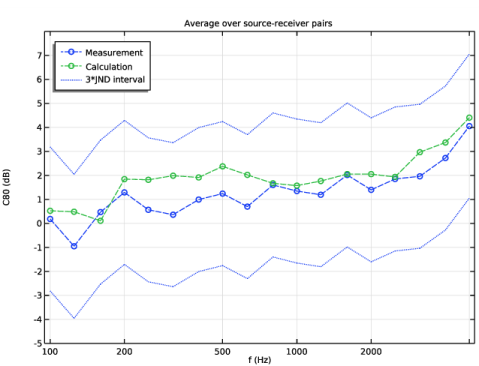
In the associated text field, type C80 (dB).
|
|
11
|
|
12
|
|
13
|
|
14
|
|
15
|
|
16
|
|
17
|
|
1
|
|
2
|
|
4
|
|
5
|
Click to expand the Coloring and Style section. Find the Line style subsection. From the Line list, choose Dashed.
|
|
6
|
|
7
|
|
8
|
|
1
|
|
2
|
|
4
|
|
5
|
Locate the Coloring and Style section. Find the Line style subsection. From the Line list, choose Dotted.
|
|
6
|
|
7
|
|
1
|
|
2
|
|
4
|
|
5
|
Locate the Coloring and Style section. Find the Line style subsection. From the Line list, choose Dotted.
|
|
6
|
|
7
|
|
8
|
|
1
|
|
2
|
|
3
|
Locate the Data section. From the Dataset list, choose Study 3 - Empty for postprocessing/Parametric Solutions 3 (sol42).
|
|
4
|
|
5
|
|
6
|
|
7
|
|
8
|
|
9
|
|
10
|
|
11
|
|
12
|
|
13
|
|
14
|
|
15
|
|
16
|
|
17
|
|
1
|
|
2
|
|
4
|
|
5
|
Click to expand the Coloring and Style section. Find the Line style subsection. From the Line list, choose Dashed.
|
|
6
|
|
7
|
|
8
|
|
1
|
|
2
|
|
4
|
|
5
|
Locate the Coloring and Style section. Find the Line style subsection. From the Line list, choose Dotted.
|
|
6
|
|
7
|
|
1
|
|
2
|
|
4
|
|
5
|
Locate the Coloring and Style section. Find the Line style subsection. From the Line list, choose Dotted.
|
|
6
|
|
7
|
|
8
|
|
1
|
|
2
|
|
3
|
Click
|
|
4
|
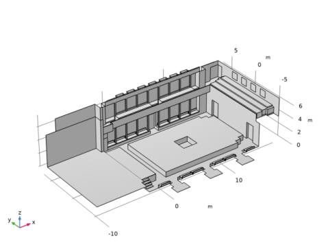
Browse to the model’s Application Libraries folder and double-click the file chamber_music_hall.mphbin.
|
|
5
|
Click
|
|
6
|
|
1
|
|
2
|
On the object imp1, select Boundary 238 only.
|
|
3
|
|
1
|
|
2
|
|
3
|
On the object ext1, select Boundaries 197, 213, 408, 419, and 661 only.
|
|
4
|
|
1
|
|
2
|
On the object ext2, select Boundary 724 only.
|
|
3
|
|
1
|
|
2
|
On the object ext3, select Boundary 746 only.
|
|
3
|
|
1
|
|
2
|
|
3
|
On the object ext4, select Boundaries 240, 252, 300, 359, 481, 543, and 597 only.
|
|
4
|
|
5
|
On the object ext4, select Boundaries 228, 240, 252, 282, 300, 341, 359, 481, 543, and 597 only.
|
|
6
|
|
7
|
On the object ext4, select Boundaries 228, 240, 252, 282, 300, 341, 359, 460, 481, 519, 543, 582, and 597 only.
|
|
8
|
|
9
|
On the object ext4, select Boundaries 199, 220, 228, 240, 252, 282, 300, 341, 359, 436, 452, 460, 481, 519, 543, 582, and 597 only.
|
|
10
|
|
11
|
On the object ext4, select Boundaries 199, 220, 228, 240, 252, 282, 300, 341, 359, 436, 452, 460, 481, 519, 543, 582, 597, 712, 714, 721, 723, 725, 742–744, 746, 750, 754, 755, and 760 only.
|
|
12
|
|
13
|
On the object ext4, select Boundaries 199, 220, 228, 240, 252, 282, 300, 341, 359, 436, 452, 460, 481, 519, 543, 582, 597, 712, 714, 721, 723, 725, 742–746, 750, 751, 754, 755, and 760 only.
|
|
14
|
|
1
|
|
2
|
|
3
|
|
4
|
|
5
|
In the Paste Selection dialog box, type del1: 1-196, 198, 201-216, 218, 220, 222-245, 250-387, 389-397, 399-410, 413, 415-424, 426, 429-439, 441, 443, 445-476, 478-609, 611-632, 634, 639, 644-680, 682-694, 699-702, 706, 708-713, 716, 718, 724-730 in the Selection text field.
|
|
6
|
Click OK.
|
|
1
|
|
2
|
|
3
|
|
4
|
|
5
|
|
6
|
Click OK.
|
|
1
|
|
2
|
|
3
|
|
4
|
|
5
|
|
6
|
Click OK.
|
|
1
|
|
2
|
|
3
|
|
4
|
|
5
|
In the Paste Selection dialog box, type del1: 158, 160, 162, 164, 166-169, 195, 197, 199, 200, 205, 209, 211, 222-224, 229, 231, 232, 246-249, 257, 263, 273-275, 280, 282-289, 309, 315, 319, 321, 330-332, 337, 339-346, 370, 376, 379, 381, 388, 411, 412, 414, 425, 427, 428, 445-447, 452, 454, 455, 459-464, 477, 482, 488, 492, 494, 502-504, 509, 511, 512, 516, 517, 521-524, 541, 547, 551, 553, 560, 561, 565, 570, 572, 573, 591, 597, 607, 608, 610, 613, 616, 618-621, 625-628, 635-638, 640-643, 681, 695-698, 703-705, 707, 714, 715, 717, 719-723 in the Selection text field.
|
|
6
|
Click OK.
|
|
1
|
|
2
|
|
3
|
|
4
|
|
5
|
In the Paste Selection dialog box, type del1: 12, 96, 98-107, 109-115, 117, 119, 122, 126, 132, 135-140, 142, 146, 150, 154, 155, 184, 185, 188, 190, 193, 298, 300, 304, 363, 365, 368, 390, 393, 396, 397, 408, 413, 473, 475, 476, 534, 536, 539, 612, 617, 622, 624, 631, 632, 639, 659, 677, 684, 685, 699-702, 706, 712, 713, 716, 718, 730 in the Selection text field.
|
|
6
|
Click OK.
|
|
1
|
|
2
|
|
3
|
|
4
|
|
5
|
In the Paste Selection dialog box, type del1: 2, 8, 97, 120, 127, 143, 152, 181, 186, 191, 238, 241, 250, 252, 295, 301, 305, 307, 352, 355, 359, 361, 366, 400, 403, 407, 415, 417, 456, 470, 478, 480, 513, 518, 530, 532, 537, 562, 574, 584, 586, 646, 647, 649, 650, 652, 653, 655, 656, 663, 690, 693, 709 in the Selection text field.
|
|
6
|
Click OK.
|
|
1
|
|
2
|
|
3
|
|
4
|
|
5
|
In the Paste Selection dialog box, type del1: 1, 3-7, 9, 108, 121, 128-131, 145, 148, 149, 151, 153, 171-180, 182, 187, 198, 201-204, 206, 208, 212-216, 218, 220, 225, 227, 233, 235, 239, 243, 251, 253, 259-262, 264, 266-272, 276, 278, 290, 292, 296, 303, 306, 308, 311-314, 316, 318, 323, 324, 326-329, 333, 335, 347, 349, 353, 357, 358, 360, 362, 372-375, 377, 378, 382-387, 389, 391, 392, 394, 395, 399, 401, 405, 416, 418, 426, 429-439, 441, 443, 448, 450, 457, 465, 467, 472, 479, 481, 484-487, 489, 491, 496-501, 505, 507, 514, 520, 525, 527, 531, 533, 543-546, 548, 550, 554-559, 563, 566, 568, 576, 577, 579, 585, 587, 593-596, 598, 600-606, 611, 614, 615, 629, 630, 634, 680, 711 in the Selection text field.
|
|
6
|
Click OK.
|
|
7
|
|
8
|