Small Concert Hall Acoustics

Designing structures and open spaces with respect to sound quality is important for concert halls, outdoor environments, and even the rooms of a house. Simulating acoustics in the high-frequency limit, where the wavelength is smaller than the geometrical features, is best done with ray acoustics.

This tutorial model shows the basic steps and principles used when setting up a model using the Ray Acoustics physics interface. In the model, the acoustics of a small concert hall is analyzed. The model setup includes an omnidirectional sound source, wall boundary conditions for specular and diffuse scattering, surface sound pressure level evaluation, analyzing the impulse response, evaluation of objective room acoustic metrics, and a reflectogram. The metric results are compared to simple analytical estimates.

Model Definition

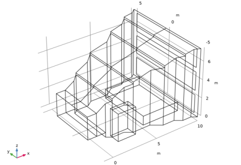
In this model the acoustics of a generic small concert hall is analyzed. Its geometry is depicted in Figure 1. It is a fan-shaped hall with a volume of 460 m3 and a total surface area of 390 m2, fitted with absorbers and diffusers. The location of the different materials is not particularly optimized and does not necessarily follow design rules. Rather than accuracy, the aim of this tutorial is to describe the important modeling steps to perform a room acoustics simulation using ray tracing. The back wall of the room consists of windows and reflective surfaces only, with all the absorption and diffusion being located on the side walls. The stage lies 0.5 m above the ground. The seating area is modeled as a box extruding 1 m high from the ground. It is common practice in ray acoustics to simplify geometry details, and seating is typically represented as a box with equivalent absorption and scattering.

An omnidirectional source is located at the coordinates (xs, ys, zs) at the front of the stage. It generates a pulse that has an SPL of 100 dB at 1 m from the source. The receiver (microphone) is located at the coordinates (xr, yr, zr). These are parameters found under . The location of the receiver can be changed in postprocessing, while the location of the source needs to be changed before running the model. The size of the receiver is set to match the common width of a seat, with a receiver radius r = 0.3 m. This value is entered on the dataset with the option . The number of rays emitted by the source is then determined to limit the error in the calculated impulse response. For an expected error of 1 dB in every time interval Δt of the response, the number of rays should be (see Ref. 1)

(1)

With Δt = 0.01 s, the resulting value gives Nrays = 9000 after rounding up. Determining the number of rays from the volume of the room and the receiver size is a favorable option as default and when there are multiple receivers in the space. Nevertheless, it is also possible to set a desired number of rays and use the predefined expression to calculate the size of the receiver according to the volume of the room, the distance to the source, and the number of rays. This corresponds to the option on the dataset. This option can be an interesting approach in the case of a single receiver.

Figure 1: Geometry of the small concert hall.

The absorption properties of the various surfaces (floor, walls, windows, seating, entrance, absorbers, and diffusers) are values taken from Ref. 1-3. The windows are taken as large panes of heavy glass, and the seating area is considered unoccupied. The data is given in octave bands and imported from the file small_concert_hall_absorption_parameters.txt into an interpolation function (lookup table). The scattering coefficients of the diffusers and seating areas are also taken from Ref. 3. For seemingly flat surfaces, a default scattering coefficient s = 0.05 is defined to account for the roughness of the materials. Moreover, the amplitude attenuation of air at 20°C and 50% humidity is imported from the file small_concert_hall_air_attenuation.txt. The imported parameter aair can be entered directly in the section, as an amplitude attenuation αext = aair(f0).

Results and Discussion

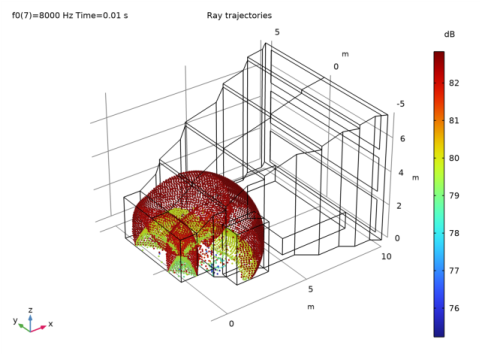
The local wavefront sound pressure level (SPL) is depicted in Figure 2 after 10 ms and in Figure 3 after 20 ms propagation for the 8 kHz frequency band. This type of plot can be used to inspect holes in the geometry and potential standing wave patterns. When the compute intensity option is selected in the Ray Acoustics interface, wavefront curvature, intensity, and SPL is calculated along each ray. They allow visualization of the (spatially) local acoustic properties. However, it is the acoustic power transported by each ray that is important when calculating the impulse response (IR) and when visualizing the sound pressure level at surfaces. This means that the compute power option should always be selected for IR computation, while the compute intensity can be turned off. Only selecting will also reduce the number of degrees of freedom (DOFs) solved for, making the model run faster and the size of the saved file smaller. The option is also necessary when analyzing the IR.

Figure 2: Ray location and SPL after 10 ms.

Figure 3: Ray location and SPL after 20 ms.

The temporal impulse response (IR) for the source and receiver configuration used in the model is depicted in Figure 4. The frequency domain (FFT) of the IR is depicted in Figure 5. The curve is smoothed with a 1/3-octave running average.

When an IR is reconstructed from a ray tracing simulation, information is inferred and put back into the time signal using the temporal filter kernels. The quality of the simulated IR increases with the number of rays as well as the frequency resolution of the absorption, scattering, and source data (this data can be difficult to get from vendors but can often be simulated). In this model, octave band resolution is used. The Impulse Response plot also allows the use of 1/3-octave and 1/6-octave frequency resolution.

Figure 4: Temporal impulse response computed at the receiver location.

Figure 5: FFT of the impulse response (1/3-octave running average).

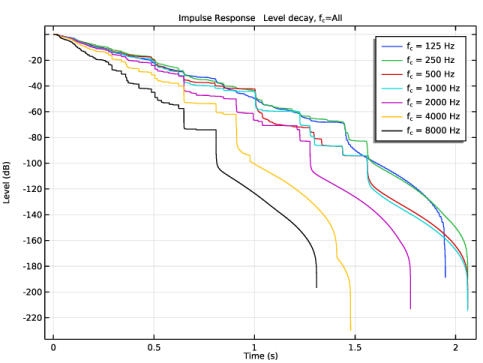
The IR is further analyzed using the subfeature to the plot. The feature allows the computation of the objective room acoustic metrics like clarity C80, definition D, early decay time EDT, center time ts, reverberation times T20, T30, T60, and speech transmission index STI. The level decay curves for the 7 octave bands used in the model (computed by the subfeature) are depicted in Figure 6. The metrics can be found in the table in the model (). The values are depicted graphically in Figure 9 and Figure 10.

Figure 6: Level decay curves for the 7 octave bands used in the model.

In order to obtain accurate room acoustic metrics, it is important to ensure the quality of the level decay curves from which they are calculated. The first indicator for quality is the smoothness of the curves. If there are flat sections followed by sudden large drops in level, the number of rays in the simulation should be increased. The default value given in Equation 1 should be sufficient for this in the majority of cases. The second aspect to look at is the amplitude of level decay before the termination point where the curves become vertical and fade out. There should indeed be a large enough decay to fit the definitions of the different room acoustic metrics (for example, T60 takes into account the decay from -5 dB to -65 dB). A general guideline for this to be true is to set the impulse response duration approximately equal to or larger than the reverberation time. This is done in , where the entered values should be 0 and the end time of the simulation. The other parameter controlling the decay amplitude is the energy threshold at which rays are terminated. This threshold should be sufficiently low to avoid losing valuable information. Its value is found in , where the default recommendation is to use as and a threshold equal to P0/Nrays·10-6. This expression ensures a consistent termination criterion according to the source power and number of rays in the simulation, with the factor 10-6 allowing a large enough decay in most cases.

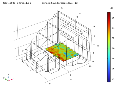
The sound pressure level on the seating area is depicted in Figure 7 for the 8 kHz band. It is calculated using the feature, available as a subnode to all boundary conditions. In this case it is added to the top surface of the box representing the seating area. The feature can be added to all other walls to postprocess the SPL distribution if necessary.

Figure 7: SPL at the location of the audience.

In the ray tracing method, the intensity I and RMS pressure prms of the nth ray detected by the receiver sphere is expressed as

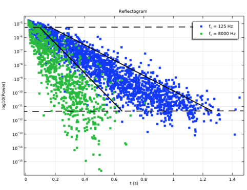
where Vr is the receiver volume, Lr is the distance traveled by the ray inside the receiver, and Qn is the power carried by the ray (see Ref. 4). The intensity is evaluated using the expression re1dist*rac.Q/re1vol. Plotting this information in a plot as a function of the arrival time yields the (discrete time) energy impulse response or reflectogram. It is plotted for the 125 Hz and the 8 kHz octave bands in Figure 8. The slope of the curves (point data) gives a visual indication of the reverberation time of the room. In Figure 8 approximate trend lines have been added manually; their slope (from -5 dB to -65 dB which is 6 decades for log10(In)) gives an estimate of the T60 reverberation time. In this case about 0.6 s for the 8 kHz band and 1.1 s for the 125 Hz band. These values are seen to fit well with the computed values below.

Figure 8: The raw data of the energetic impulse response or reflectogram. The slope represents the reverberation time in the given octave band.

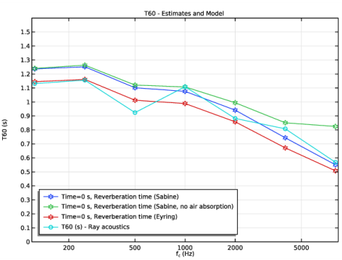
A comparison between the computed value of reverberation time and simple statistical estimates is shown in Figure 9. To plot the data from the results table the plot is used. The estimated values are calculated using the Sabine and Eyring equations used in statistical room acoustics

where V is the room volume, S is the total surface area, aair is the atmospheric amplitude attenuation, and

is the average wall absorption (see Ref. 2). The results show a good agreement in this case. However, it is not expected that the Sabine and Eyring predictions always match simulation results closely, especially in rooms where the diffuse sound field assumption does not hold.

Figure 9: Reverberation time estimates based on the Sabine and Eyring formulas compared to the computed reverberation time.

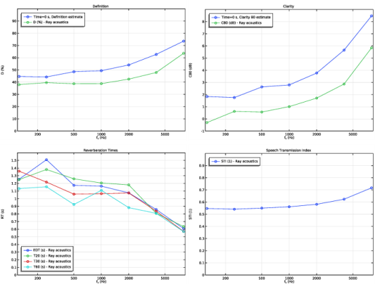
Selected room acoustic metrics are plotted as functions of the octave band center frequency in Figure 10. The definition, the clarity, and the center time metrics are also compared to analytical estimates in the figures. The estimates are based on analytical models of the direct energy, early energy, and late energy (see Ref. 1). They are defined in the .

Definition D (or D50) gives a metric for syllable intelligibility. In this room it is around 40% for most bands which is acceptable for a space with a purpose focused on music. The clarity metric C80 is used to characterize the transparency of music, for concert halls typical values lie between -5 to +3 dB. In this case the design is not optimal for the higher octave bands. The center time is another metric that correlates to speech intelligibility, it is not shown here but can be found in the model. All metrics should be estimated taking their just noticeable difference (JND) into account.

The speech transmission index STI is a single valued metric for speech intelligibility. It is based on modulation transfer function values (14 frequencies) and 7 octave bands. The can be plotted using the subfeature. The STI is computed as a single value that combines the information in the 7 bands. To get the single metric, change the to in the plot. Making these changes gives an STI value of 0.59 (this indicates good intelligibility). The STI values plotted as a function of octave band center frequency in Figure 10 are computed based on the apparent signal to noise ratio in each band. When is selected the values in the different bands contribute with the appropriate weighting.

Figure 10: Objective room acoustic metrics clarity, definition, reverberation times, and speech transmission index plotted as functions of octave band center frequency. The clarity and definition metrics are compared to analytical estimates. The center time (not shown here) can be seen in the plots in the model.

Notes About the COMSOL Implementation

There are several options that can be selected on the node that are useful when working with ray acoustic models and especially when evaluating the impulse response.

•

When first setting up plots, it is useful to select the option as some plots take a long time to render. Another trick is to use only a few rays initially.

•

Once the plots are set up, then before running the model (with a large number of rays), select the option. Once the model has solved the plots will be rendered. This is very useful when running the model over lunch break or over night since rendering the IR plot often takes longer time than solving the model.

•

Before saving the model, remember to set the list to . Then all plots do not need to be re-rendered once the model is opened again.

References

1. M. Vorländer, Auralization, Fundamentals of Acoustics, Modeling, Simulation, Algorithms and Acoustic Virtual Reality, Springer, 2008.

2. H. Kuttruff, Room Acoustics, CRC Press, 2009.

3. T. J. Cox and P. D’Antonio, Acoustic Absorbers and Diffusers: Theory, design and application, Taylor & Francis, 2009.

4. Z. Xiangyang, C. Ke’an, and S. Jincai, “On the accuracy of the ray-tracing algorithms based on various sound receiver models,” Appl. Acoust., vol. 64, pp. 433–441, 2003.

Acoustics_Module/Building_and_Room_Acoustics/small_concert_hall

Modeling Instructions

This section contains the modeling instructions for the Small Concert Hall model. They are followed by the Geometry Modeling Instructions section.

From the menu, choose .

New

In the window, click

Model Wizard

In the window, click

In the tree, select .

Click .

Click

In the tree, select .

Click

Geometry 1

The geometry is set up by importing a geometry sequence. The sequence imports the small concert hall geometry and sets up several selections. The predefined selections simplify the rest of the model setup.

In the toolbar, click and choose .

Browse to the model’s Application Libraries folder and double-click the file small_concert_hall_geom_sequence.mph.

In the toolbar, click

Click the

button in the toolbar.

Click the

button in the toolbar.

Import the model parameters from the files. The parameters include the band center frequency f0, the location of the source and receiver, as well as the room volume.

Global Definitions

Parameters 1 - Model

In the window, under click .

In the window for , type Parameters 1 - Model in the text field.

Locate the section. Click

Browse to the model’s Application Libraries folder and double-click the file small_concert_hall_parameters_model.txt.

Parameters 2 - Source and receiver positions

In the toolbar, click

and choose .

In the window for , type Parameters 2 - Source and receiver positions in the text field.

Locate the section. Click

Browse to the model’s Application Libraries folder and double-click the file small_concert_hall_parameters_source_positions.txt.

Parameters 3 - Source and receiver settings

In the toolbar, click

and choose .

In the window for , type Parameters 3 - Source and receiver settings in the text field.

Locate the section. Click

Browse to the model’s Application Libraries folder and double-click the file small_concert_hall_parameters_source_settings.txt.

Proceed and set up interpolation functions for the absorption coefficients of the different surfaces in the concert hall. The data is easily stored in one .txt file. Also define an interpolation function for the amplitude attenuation of air (given at 50% relative humidity and 20°C).

Interpolation 1 (int1)

In the toolbar, click

and choose .

In the window for , locate the section.

From the list, choose .

Click

Browse to the model’s Application Libraries folder and double-click the file small_concert_hall_absorption_parameters.txt.

In the text field, type 1.

Click

Find the subsection. In the table, enter the following settings:


Function name	Position in file
a_walls	1
a_entrance	2
a_windows	3
a_floor	4
a_diffuser	5
a_seats	6
a_absorbers	7

Locate the section. From the list, choose .

Locate the section. In the table, enter the following settings:


Function	Unit
a_walls	1
a_entrance	1
a_windows	1
a_floor	1
a_diffuser	1
a_seats	1
a_absorbers	1

In the table, enter the following settings:


Argument	Unit
Column 1	Hz

Interpolation 2 (int2)

In the toolbar, click

and choose .

In the window for , locate the section.

From the list, choose .

Click

Browse to the model’s Application Libraries folder and double-click the file small_concert_hall_air_attenuation.txt.

Click

In the text field, type a_air.

Locate the section. From the list, choose .

Locate the section. In the table, enter the following settings:


Argument	Unit
t	Hz

In the table, enter the following settings:


Function	Unit
a_air	1/m

Now import the variables that define the room acoustic quality metric estimates. They include the reverberation time (T60), based on the Sabine and Eyring estimation equations, clarity, definition, and center time. This also requires setting up integration operators for all the surfaces.

Definitions

Integration 1 (intop1)

In the window, expand the node.

Right-click and choose .

In the window for , type intop_windows in the text field.

Locate the section. From the list, choose .

From the list, choose .

Integration 2 (intop2)

In the toolbar, click

and choose .

In the window for , type intop_seats in the text field.

Locate the section. From the list, choose .

From the list, choose .

Integration 3 (intop3)

In the toolbar, click

and choose .

In the window for , type intop_diffusers in the text field.

Locate the section. From the list, choose .

From the list, choose .

Integration 4 (intop4)

In the toolbar, click

and choose .

In the window for , type intop_floor in the text field.

Locate the section. From the list, choose .

From the list, choose .

Integration 5 (intop5)

In the toolbar, click

and choose .

In the window for , type intop_entrance in the text field.

Locate the section. From the list, choose .

From the list, choose .

Integration 6 (intop6)

In the toolbar, click

and choose .

In the window for , type intop_walls in the text field.

Locate the section. From the list, choose .

From the list, choose .

Integration 7 (intop7)

In the toolbar, click

and choose .

In the window for , type intop_absorbers in the text field.

Locate the section. From the list, choose .

From the list, choose .

Variables: Quality Metric Estimates

Right-click and choose .

In the window for , type Variables: Quality Metric Estimates in the text field.

Locate the section. Click

Browse to the model’s Application Libraries folder and double-click the file small_concert_hall_variables.txt.

Proceed to set up and define the physics and boundary conditions of the model. To compute the impulse response, it is necessary to model the power along the rays and count the reflections. In the model the intensity is also computed along the rays. The intensity represents spatially local properties of the acoustic field approximated by the rays. The model only uses a surface mesh. Propagation in the unmeshed domains requires the definition of material properties at the interface level (in the section ). Set up boundary conditions for the different walls. All the boundary conditions are defined as , with either a default or specific scattering coefficient.

Ray Acoustics (rac)

In the window, under click .

In the window for , locate the section.

From the list, choose .

Locate the section. In the cext text field, type c0.

In the ρext text field, type rho0.

In the αext text field, type a_air(f0).

Locate the section. Select the check box.

Ray Properties 1

In the window, under click .

In the window for , locate the section.

In the f text field, type f0.

Wall: Walls

In the toolbar, click

and choose .

In the window for , type Wall: Walls in the text field.

Locate the section. From the list, choose .

In the γs text field, type 1-s_default.

Locate the section. In the αs text field, type a_walls(f0).

In the αd text field, type a_walls(f0).

Wall: Entrance

In the toolbar, click

and choose .

In the window for , type Wall: Entrance in the text field.

Locate the section. From the list, choose .

In the γs text field, type 1-s_default.

Locate the section. In the αs text field, type a_entrance(f0).

In the αd text field, type a_entrance(f0).

Wall: Windows

In the toolbar, click

and choose .

In the window for , type Wall: Windows in the text field.

Locate the section. From the list, choose .

In the γs text field, type 1-s_default.

Locate the section. In the αs text field, type a_windows(f0).

In the αd text field, type a_windows(f0).

Wall: Floor

In the toolbar, click

and choose .

In the window for , type Wall: Floor in the text field.

Locate the section. From the list, choose .

In the γs text field, type 1-s_default.

Locate the section. In the αs text field, type a_floor(f0).

In the αd text field, type a_floor(f0).

Wall: Diffusers

In the toolbar, click

and choose .

In the window for , type Wall: Diffusers in the text field.

Locate the section. From the list, choose .

In the γs text field, type 1-s_diffuser.

Locate the section. In the αs text field, type a_diffuser(f0).

In the αd text field, type a_diffuser(f0).

In this model the scattering coefficient s_diffuser is constant across the frequency bands. It can of course also be defined as an interpolation function that depends on f0.

Wall: Absorbers

In the toolbar, click

and choose .

In the window for , type Wall: Absorbers in the text field.

Locate the section. From the list, choose .

In the γs text field, type 1-s_default.

Locate the section. In the αs text field, type a_absorbers(f0).

In the αd text field, type a_absorbers(f0).

Wall: Seats (top)

In the toolbar, click

and choose .

In the window for , type Wall: Seats (top) in the text field.

Locate the section. From the list, choose .

Select Boundary 41 only.

Locate the section. From the list, choose .

In the γs text field, type 1-s_seats.

Locate the section. In the αs text field, type a_seats(f0).

In the αd text field, type a_seats(f0).

Sound Pressure Level Calculation 1

In the toolbar, click

and choose .

In the window for , locate the section.

Select the check box.

Wall: Seats (around)

In the toolbar, click

and choose .

In the window for , type Wall: Seats (around) in the text field.

Locate the section. From the list, choose .

Select Boundaries 39, 40, 42, and 59 only.

Locate the section. From the list, choose .

In the γs text field, type 1-s_seats.

Locate the section. In the αs text field, type a_seats(f0).

In the αd text field, type a_seats(f0).

Release from Grid 1

In the toolbar, click

and choose .

In the window for , locate the section.

In the qx,0 text field, type x_s.

In the qy,0 text field, type y_s.

In the qz,0 text field, type z_s.

Locate the section. From the list, choose .

In the Nw text field, type Nrays.

Locate the section. In the Psrc text field, type P0.

Ray Termination 1

In the toolbar, click

and choose .

In the window for , locate the section.

From the list, choose .

In the Qth text field, type P0/Nrays*1e-6.

Mesh 1

In the window, under click .

In the window for , locate the section.

From the list, choose .

Size

In the window, under click .

In the window for , locate the section.

From the list, choose .

Free Triangular 1

In the window, click .

In the window for , locate the section.

From the list, choose .

Size 1

Right-click and choose .

Add a finer mesh on the surface where the SPL is computed.

In the window for , locate the section.

Click

Select Boundary 41 only.

Locate the section. Click the button.

Locate the section. Select the check box.

In the associated text field, type 0.3.

Click

Proceed and solve the model by adding a parametric sweep over the center frequency variable f0. This represents the center frequency of the octave bands analyzed in this model, in order to get a broadband response. The first time you set up and solve the model it can be useful to reduce the number of rays by changing the value of the parameter Nrays to, for example, 1000. This will make solving and postprocessing faster. Remember that the quality of the results in acoustic ray tracing increase for an increasing number of rays and more narrow frequency bands (you need to have wall absorption data with the desired resolution). In the Ray Acoustics interface the impulse response plot can handle octave, 1/3-octave, and 1/6-octave data.

Study 1

Step 1: Ray Tracing

In the window, under click .

In the window for , locate the section.

From the list, choose .

In the text field, type 0 1.6.

For optimal performance only enter 0 and the end time for the simulation. In postprocessing, when reconstructing the impulse response, additional exact time steps for all the wall reflections are used and rendered.

Parametric Sweep

In the toolbar, click

Using the parametric sweep is important as this gives the frequency resolution (here in full octaves). The ray propagation model is solved once per frequency band. The data is collected in postprocessing, by the receiver dataset and the impulse response plot, to generate the broadband impulse response.

In the window for , locate the section.

Click

In the table, click to select the cell at row number 1 and column number 2.

In the table, enter the following settings:


Parameter name	Parameter value list	Parameter unit
f0 (Band center frequency)		Hz

Click

In the dialog box, choose from the list.

In the text field, type 125.

In the text field, type 8000.

Click .

Solving the model takes a couple of minutes and uses less than 4 GB of RAM (depending on your hardware). This will increase for an increasing number of rays.

In the toolbar, click

Results

Ray Trajectories (rac)

In the window for , locate the section.

From the list, choose .

In the text field, type 10[ms].

In the toolbar, click

Ray Trajectories 1

In the window, expand the node, then click .

In the window for , locate the section.

Find the subsection. From the list, choose .

Color Expression 1

In the window, expand the node, then click .

In the window for , locate the section.

In the text field, type rac.Lp.

In the toolbar, click

This should reproduce the image in Figure 2.

Ray Trajectories (rac)

In the window, under click .

In the window for , locate the section.

In the text field, type 20[ms].

In the toolbar, click

This should reproduce the image in Figure 3.

On the node you have several options that are useful when postprocessing ray tracing simulations, where rendering plots can be time consuming. This is especially true for the impulse response plots. While setting up plots, it is useful to select such that the plots are not generated every time you change an option. It is also good practice to save the plots in the model such that they are already rendered when you open your model at a later stage. Finally, once you have set up all the plots and you are ready to run the model again, it can be useful to enable . All plots will then be recomputed after the model is solved, for example, running over lunch.

In the window, click .

In the window for , locate the section.

Select the check box.

Locate the section. From the list, choose .

Also turn on the to display rendering time and other useful information. This option applies to the whole COMSOL installation; if selected, the will also appear in other models opened at a later stage.

Click the

button in the toolbar.

In the dialog box, select in the tree.

In the tree, select the check box for the node .

Click .

Now set up the dataset used for creating the impulse response and subsequent analysis.

Receiver 3D - All Bands

In the window, expand the node.

Right-click and choose .

In the window for , type Receiver 3D - All Bands in the text field.

Locate the section. Find the subsection. In the text field, type x_r.

In the text field, type y_r.

In the text field, type z_r.

Find the subsection. From the list, choose .

In the text field, type r_rec.

The default recommendation is to use a receiver radius of 0.3 m, which corresponds to the standard width of a seat. For different applications, especially smaller spaces like a car cabin, it is recommended to decrease the value of the receiver radius.

Receiver 3D - 125 Hz Band

In the window, right-click and choose .

In the window for , type Receiver 3D - 125 Hz Band in the text field.

Locate the section. From the list, choose .

In the list, select .

Receiver 3D - 8 kHz Band

In the window, right-click and choose .

In the window for , type Receiver 3D - 8 kHz Band in the text field.

Locate the section. From the list, choose .

In the list, select .

Impulse Response

In the toolbar, click

In the window for , type Impulse Response in the text field.

Locate the section. From the list, choose .

Impulse Response 1

In the toolbar, click

and choose .

To get sharper filters you can modify some settings in the section.

In the window for , click to expand the section.

In the Np text field, type 22050.

In the δ text field, type 0.001.

Rendering the impulse response will typically take one or two minutes (depending on hardware, number of rays, and frequency band resolution). Once the plot has been generated (the first time) the necessary ray data is cached and any subsequent changes/updates of the plot is faster. The rendering time for the last time a figure was plotted can be found in the first subnode of its plot group, under in the window.

In the toolbar, click

This should reproduce the impulse response shown in Figure 4. The impulse response is the most important result of this model. The signal can be exported under the Export node and used for further analysis in an external signal processing tool. The response is reconstructed from the ray data detected by the Receiver dataset (arrival time, power, and band center frequency). It has a default sampling frequency of 44100 Hz. This can also be changed under the Advanced section in the plot settings window.

Plot 1

Right-click and choose .

In the window for , locate the section.

From the list, choose .

In the text field, type small_concert_hall_impulse_response.wav.

Click to expand the section. From the list, choose .

Click to produce a wav file with the impulse response. This file could be used for auralization or analysis with other tools. Remember to disable any subfeature before exporting.

Proceed to analyze the impulse response with the subfeature. This will create a plot of the level/energy decay and a table with the objective quality metrics.

Energy Decay 1

In the window, expand the node.