|
|
|
|
1
|
|
2
|
|
3
|
Click Add.
|
|
4
|
Click
|
|
5
|
|
6
|
Click
|
|
1
|
|
2
|
|
3
|
|
1
|
|
2
|
|
3
|
|
1
|
|
2
|
|
3
|
|
4
|
|
5
|
|
6
|
|
1
|
|
2
|
|
3
|
|
4
|
|
5
|
|
6
|
|
1
|
|
2
|
|
3
|
|
4
|
|
5
|
|
6
|
|
1
|
|
2
|
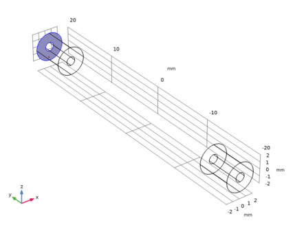
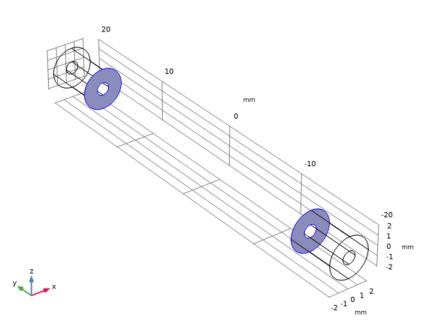
Select the object cyl1 only.
|
|
3
|
|
4
|
|
5
|
|
6
|
|
1
|
In the Model Builder window, under Component 1 (comp1) right-click Materials and choose Blank Material.
|
|
2
|
|
1
|
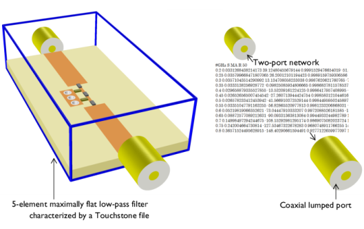
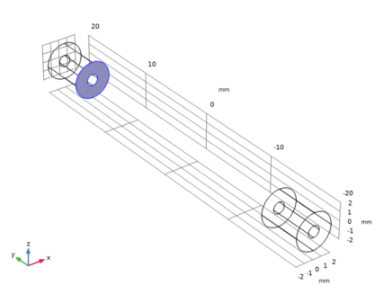
In the Model Builder window, under Component 1 (comp1) right-click Electromagnetic Waves, Frequency Domain (emw) and choose Lumped Port.
|
|
3
|
|
4
|
|
1
|
|
2
|
|
4
|
|
5
|
|
1
|
|
1
|
In the Model Builder window, expand the Two-Port Network 1 node, then click Two-Port Network Port 1.
|
|
1
|
|
1
|
|
2
|
|
3
|
|
4
|
|
5
|
Click Browse.
|
|
6
|
Browse to the model’s Application Libraries folder and double-click the file two_port_network_touchstone.s2p.
|
|
7
|
Click Import.
|
|
8
|
|
1
|
|
2
|
|
3
|
|
4
|