PDF

DC Glow Discharge Coupled with the Two-Term Boltzmann Equation
Introduction
DC glow discharges in the low pressure regime have long been used for gas lasers and fluorescent lamps. DC discharges are attractive to study because the solution is time independent. This model shows how to use the Plasma interface to set up an analysis of a positive column. The discharge is sustained by emission of secondary electrons at the cathode.
This tutorial models a DC discharge by solving plasma fluid equations fully coupled with the homogeneous and time-independent electron Boltzmann equation in the classical two-term approximation. The approximated Boltzmann equation is solved for each position of space and is coupled with the fluid equations by way of the electron mean energy. The rate constants of electron impact reactions and the electron transport parameters are obtained by suitable integration of the computed electron energy distribution function over electron scattering cross sections. Simulation results from this model are compared with results from the model DC Glow Discharge, 1D where the electron energy distribution function (EEDF) is assumed to be Maxwellian.
Model Definition
The DC discharge consists of two electrodes, one powered (the anode) and one grounded (the cathode):
Figure 1: Schematic of the DC discharge. The voltage applied across the electrodes leads to formation of a plasma.
domain equations
The electron density and mean electron energy are computed by solving a pair of drift-diffusion equations for the electron density and mean electron energy. Convection of electrons due to fluid motion is neglected. For detailed information on electron transport see Theory for the Drift Diffusion Interface in the Plasma Module User’s Guide.
where:
The electron source Re and the energy loss due to inelastic collisions Rε are defined later. The electron diffusivity, energy mobility and energy diffusivity are computed from the electron mobility using:
The source coefficients in the above equations are determined by the plasma chemistry using rate coefficients. Suppose that there are M reactions which contribute to the growth or decay of electron density and P inelastic electron-neutral collisions. In general P >> M. In the case of rate coefficients, the electron source term is given by:
where xj is the mole fraction of the target species for reaction j, kj is the rate coefficient for reaction j (m3/s), and Nn is the total neutral number density (1/m3). For DC discharges it is better practice to use Townsend coefficients instead of rate coefficients to define reaction rates. Townsend coefficients provide a better description of what happens in the cathode fall region Ref 1. When Townsend coefficients are used, the electron source term is given by:
where αj is the Townsend coefficient for reaction j (m2) and Γe is the electron flux as defined above (1/(m2·s)). Townsend coefficients can increase the stability of the numerical scheme when the electron flux is field driven as is the case with DC discharges. The electron energy loss is obtained by summing the collisional energy loss over all reactions:
where Δεj is the energy loss from reaction j (V). When Townsend coefficients are used, the electron energy loss is taken as:
.
For non-electron species, the following equation is solved for the mass fraction of each species. For detailed information on the transport of the non-electron species see Theory for the Heavy Species Transport Interface in the Plasma Module User’s Guide.
The electrostatic field is computed using the following equation:
The space charge density ρ is automatically computed based on the plasma chemistry specified in the model using the formula:
For detailed information about electrostatics see Theory for the Electrostatics Interface in the Plasma Module User’s Guide.
Boltzmann Equation in the Two-Term Approximation
The EEDF used in this model is obtained from the solution of the homogeneous and time-independent electron Boltzmann equation in the classical two-term approximation
where F0 is the isotropic part of an EEDF constant in time and space that verifies the following normalization
.
The different terms are presented below:
The following definitions apply
.
Here:
γ = (2q/me)1/2 (SI unit: C1/2/kg1/2)
me is the electron mass (SI unit: kg)
ε = (v/γ)2 is energy (SI unit: V)
σε is the total elastic collision cross section (SI unit: m2)
σm is the total momentum collision cross section (SI unit: m2)
q is the electron charge (SI unit: C)
ε0 is the permittivity of free space (SI unit: F/m)
T is the temperature of the background gas (SI unit: K)
kb is the Boltzmann constant (SI unit: J/K)
ne is the electron density (SI unit: 1/m3)
Nn is the background gas density (SI unit: 1/m3)
λ is a scalar-valued renormalization factor that ensures that the EEDF is normalized to 1as explained above. An ODE is implemented to solve for the value of λ.
M is the mass of the target species (SI unit: kg).
The source term, S represents energy loss due to inelastic collisions. Because the energy loss due to an inelastic collision is quantized, the source term is nonlocal in the energy space. The source term can be decomposed into four parts where the following definitions apply:
where xk is the mole fraction of the target species for reaction k, σk is the collision cross section for reaction k, Δεk is the energy loss from collision k, and δ is the delta function at ε = 0.
The mean electron energy is defined by the integral
.
The external excitation in the Boltzmann equation comes from an electric field. If the Boltzmann equation is to be solved for a given mean electron energy (as in the present model) a Lagrange multiplier is introduced to solve for the reduced electric field, such that the following equation, presented in the weak form of the constraint, is satisfied:
where the tilde denotes a test function. For detailed information about electrostatics see Theory for the Boltzmann Equation, Two-Term Approximation Interface in the Plasma Module User’s Guide.
Coupling Between the Fluid Model and the Boltzmann Equation
The fluid model and the Boltzmann equation are solved fully coupled. The Boltzmann equation is solved at every point in space using as input the space dependent mean electron energy and the mole fraction of the different heavy species obtained from the fluid model. The EEDFs obtained from the solution of the Boltzmann equation are used to compute macroscopic rate constants and transport coefficients intervening in the fluid model equations thus closing the loop.
Electron Rate Coefficients, Townsend Coefficients, and Transport Parameters
Rate coefficient for electron impact reaction are computed using cross section data and computed EEDFs by the following integral
.
The Townsend coefficients are computed using
where νk is the frequency associated with the reaction rate kk
and P is the power absorbed by the electrons from the DC electric field. The reduced electron mobility is computed using
.
boundary conditions
Unlike RF discharges, the mechanism for sustaining the discharge is emission of secondary electrons from the cathode. An electron is emitted from the cathode surface with a specified probability when struck by an ion. These electrons are then accelerated by the strong electric field close to the cathode where they acquire enough energy to initiate ionization. The net result is a rapid increase in the electron density close to the cathode in a region often known as the cathode fall or Crookes dark space.
Electrons are lost to the wall due to random motion within a few mean free paths of the wall and gained due to secondary emission effects, resulting in the following boundary condition for the electron flux:
(1)
and the electron energy flux:
(2)
The second term on the right-hand side of Equation 1 is the gain of electrons due to secondary emission effects, γp being the secondary emission coefficient. The second term in Equation 2 is the secondary emission energy flux, εp being the mean energy of the secondary electrons. For the heavy species, ions are lost to the wall due to surface reactions and the fact that the electric field is directed toward the wall:
plasma chemistry
Argon is one of the simplest mechanisms to implement at low pressures. The electronically excited states can be lumped into a single species which results in a chemical mechanism consisting of only 3 species and 7 reactions (electron impact cross-sections are obtained from Ref. 3):
In this discharge, the electron density and density of excited species is relatively low so stepwise ionization is not as important as in high density discharges. In addition to volumetric reactions, the following surface reactions are implemented:
When a metastable argon atom makes contact with the wall, it reverts to the ground state argon atom with some probability (the sticking coefficient).
Results and Discussion
In this section, results are presented from the model. For reference, results of the fluid model when assuming a Maxwellian EEDF are also presented.
Figure 2 to Figure 7 present the electron density, the electron temperature, the potential, the mass fraction of the argon excited state, the current densities of the charged species, and the electron transport parameters along the discharge. All quantities presented change significantly when the EEDF is computed. In summary: the electron density is more than 50 % smaller and the maximum deviates toward the cathode; the electron temperature profile is similar but it is 1 eV higher corresponding to a increase of 50 %; the mass fraction of the argon excited is considerable different with a much more pronounced maximum near the cathode and a much smaller population in the positive column; the different current densities maintain roughly the same profile and magnitude with a difference of only10 %.
Perhaps the most important difference between the two models is the fact that the creation of excited species and ions in the positive column is much smaller for the case when the EEDF is computed. This can be verified from the plots of the source terms of these species (not presented). For the ions, the source term can be verified to be close to zero since the ion current above 20 cm is practically constant meaning that the source term is zero (the divergence of the ion flux is zero).
At a first look this might seem incoherent with the fact that the electron temperature increases for the case of the computed EEDF. However, this can be understandable by looking at the shape of the computed EEDFs in the region of the positive column presented in Figure 8. The EEDFs deviates considerable from a Maxwellian with the high energy region above the excitation and ionization thresholds being strongly unpopulated. EEDFs with these shapes when integrated over the excitation or ionization cross-section give small rate coefficients.
When modeling a DC discharge one might find that using a computed EEDF gives better agreement with experiments. By inspecting the EEDFs the use of an analytic EEDF with a depleted tail, representative of the EEDFs in positive column, might not be adequate since the EEDF in the cathode region has a different shape closer to a Maxwellian. For this case, a good option to avoid large computational times is to give to the fluid model a previously computed EEDF in the form of a lookup table as a function of the mean electron energy.
Figure 2: Electron density obtained with the present model that computes the EEDF and from the same model where the EEDF was assumed to be Maxwellian.
Figure 3: Electron temperature obtained with the present model that computes the EEDF and from the same model where the EEDF was assumed to be Maxwellian.
Figure 4: Potential obtained with the present model that computes the EEDF and from the same model where the EEDF was assumed to be Maxwellian.
Figure 5: Mass fraction of the excited argon obtained with the present model that computes the EEDF and from the same model where the EEDF was assumed to be Maxwellian.
Figure 6: Electron current density (blue), the ion current density (green), and the total current density (red) obtained with the present model that computes the EEDF and from the same model where the EEDF was assumed to be Maxwellian.
Figure 7: Reduced electron mobility (blue) and diffusivity (green) electron current density (blue), the ion current density (green) and the total current density (red) obtained with the present model that computes the EEDF and from the same model where the EEDF was assumed to be Maxwellian.
Figure 8: Computed EEDFs in the positive column region (1.9 cm) and in the cathode fall region (18 cm). For reference, it is presented a Maxwellian EEDF with the mean energy obtained from the model with the computed EEDF.
References
1. M.A. Lieberman and A.J. Lichtenberg, Principles of Plasma Discharges and Materials Processing, John Wiley & Sons, 2005.
2. G.J.M. Hagelaar and L.C. Pitchford, “Solving the Boltzmann Equation to Obtain Electron Transport Coefficients and Rate Coefficients for Fluid Models,” Plasma Sources Science and Technology, vol. 14, pp. 722–733, 2005.
3. Phelps database, www.lxcat.net, retrieved 2017.
Application Library path: Plasma_Module/Space-Dependent_EEDF_Modeling/positive_column_1d_boltzmann
Modeling Instructions
Root
The following instructions show how to create a model that solves plasma fluid type equations fully coupled with the Boltzmann equation in the two-term approximation.
The DC positive column is used as an example. Go to the Application Libraries and open the positive_column_1d model.
1
From the File menu, choose Open.
2
From the Application Libraries root, browse to the folder Plasma_Module/Direct_Current_Discharges and double-click the file positive_column_1d.mph.
Select to solve the Boltzmann equation in the two-term approximation, set the number of elements in the extra dimension to 50 and choose to compute the maximum energy automatically.
Component 1 (comp1)
In the Model Builder window, expand the Component 1 (comp1) node.
Plasma (plas)
1
In the Model Builder window, expand the Component 1 (comp1)>Plasma (plas) node, then click Plasma (plas).
2
In the Settings window for Plasma, locate the Electron Energy Distribution Function Settings section.
3
From the Electron energy distribution function list, choose Boltzmann equation, two-term approximation (linear).
4
In the N text field, type 50.
5
Select the Compute maximum energy check box.
6
Click to expand the Discretization section. From the Formulation list, choose Finite element, log formulation (linear shape function).
Change the two reactions that use Townsend coefficients from lookup tables to use cross section data and click on Use Townsend coefficient. This way the Twonsend coefficients are computed using the electron impact cross section and the computed EEDF.
2: e+Ar=>e+Ars
1
In the Model Builder window, under Component 1 (comp1)>Plasma (plas) click 2: e+Ar=>e+Ars.
2
In the Settings window for Electron Impact Reaction, locate the Collision section.
3
From the Specify reaction using list, choose Cross-section data.
4
Locate the Reaction Parameters section. Select the Use Townsend coefficient check box.
4: e+Ar=>2e+Ar+
1
In the Model Builder window, click 4: e+Ar=>2e+Ar+.
2
In the Settings window for Electron Impact Reaction, locate the Collision section.
3
From the Specify reaction using list, choose Cross-section data.
4
Locate the Reaction Parameters section. Select the Use Townsend coefficient check box.
Choose to define the transport parameters using the Mobility from electron energy distribution function. This way, the electron mobility is obtained from suitable integration of the EEDF over the cross section for momentum transfer. The remaining transport parameters are computed using the electron mobility.
Plasma Model 1
1
In the Model Builder window, click Plasma Model 1.
2
In the Settings window for Plasma Model, locate the Electron Density and Energy section.
3
From the Electron transport properties list, choose Mobility from electron energy distribution function.
Maxwellian EEDF
1
In the Model Builder window, click Study 1.
2
In the Settings window for Study, type Maxwellian EEDF in the Label text field.
Add a EEDF Initialization study to solve for the EEDF only. The solution of this study is going to be used as the initial condition for the study that solves the fluid type equations coupled with the Boltzmann equation.
Add Study
1
In the Home toolbar, click  Add Study to open the Add Study window.
2
Go to the Add Study window.
3
Find the Studies subsection. In the Select Study tree, select Preset Studies for Selected Physics Interfaces>EEDF Initialization.
4
Click Add Study in the window toolbar.
5
In the Home toolbar, click  Add Study to close the Add Study window.
EEDF Initialization
1
In the Model Builder window, click Study 2.
2
In the Settings window for Study, type EEDF Initialization in the Label text field.
3
In the Home toolbar, click  Compute.
Results
Electron Energy Distribution Function, EEDF Initialization
1
In the Settings window for 1D Plot Group, type Electron Energy Distribution Function, EEDF Initialization in the Label text field.
2
Locate the Axis section. Select the Manual axis limits check box.
3
Locate the Plot Settings section. In the x-axis label text field, type Energy (eV).
4
In the y-axis label text field, type EEDF (eV<sup>-3/2</sup>).
5
Locate the Axis section. In the x minimum text field, type 0.
6
In the x maximum text field, type 50.
7
In the y minimum text field, type 1e-8.
8
In the y maximum text field, type 1.
9
In the Electron Energy Distribution Function, EEDF Initialization toolbar, click  Plot.
Add a new study to solve for the plasma fluid type equations fully coupled with the Boltzmann equation in the two-term approximation.
Add Study
1
In the Home toolbar, click  Add Study to open the Add Study window.
2
Go to the Add Study window.
3
Find the Studies subsection. In the Select Study tree, select General Studies>Time Dependent.
4
Click Add Study in the window toolbar.
5
In the Home toolbar, click  Add Study to close the Add Study window.
Study 3
Step 1: Time Dependent
1
In the Settings window for Time Dependent, locate the Study Settings section.
2
In the Output times text field, type 0 10^{range(-8,8/100,0)}.
3
Click to expand the Values of Dependent Variables section. Find the Initial values of variables solved for subsection. From the Settings list, choose User controlled.
4
From the Method list, choose Solution.
5
From the Study list, choose EEDF Initialization, EEDF Initialization.
6
In the Model Builder window, click Study 3.
7
In the Settings window for Study, locate the Study Settings section.
8
Clear the Generate default plots check box.
9
In the Label text field, type Computed EEDF.
10
In the Home toolbar, click  Compute.
Compare the results of the model that used a Maxwellian EEDF and the on that computes the EEDF.
Results
Electron Density (plas)
1
In the Model Builder window, under Results click Electron Density (plas).
2
In the Settings window for 1D Plot Group, click to expand the Title section.
3
From the Title type list, choose None.
4
Locate the Axis section. Select the Manual axis limits check box.
5
In the y maximum text field, type 2E16.
Line Graph 1
1
In the Model Builder window, expand the Electron Density (plas) node, then click Line Graph 1.
2
In the Settings window for Line Graph, click to expand the Legends section.
3
Select the Show legends check box.
4
From the Legends list, choose Manual.
5
Line Graph 2
1
Right-click Results>Electron Density (plas)>Line Graph 1 and choose Duplicate.
2
In the Settings window for Line Graph, locate the Data section.
3
From the Dataset list, choose Computed EEDF/Solution 3 (sol3).
4
From the Time selection list, choose Last.
5
Locate the Legends section. In the table, enter the following settings:
6
In the Electron Density (plas) toolbar, click  Plot.
Results
Electron Density (plas)
In the Model Builder window, collapse the Results>Electron Density (plas) node.
Electron Temperature (plas)
1
In the Model Builder window, click Electron Temperature (plas).
2
In the Settings window for 1D Plot Group, locate the Title section.
3
From the Title type list, choose None.
Line Graph 1
1
In the Model Builder window, expand the Electron Temperature (plas) node, then click Line Graph 1.
2
In the Settings window for Line Graph, locate the Legends section.
3
Select the Show legends check box.
4
From the Legends list, choose Manual.
5
Line Graph 2
1
Right-click Results>Electron Temperature (plas)>Line Graph 1 and choose Duplicate.
2
In the Settings window for Line Graph, locate the Data section.
3
From the Dataset list, choose Computed EEDF/Solution 3 (sol3).
4
From the Time selection list, choose Last.
5
Locate the Legends section. In the table, enter the following settings:
6
In the Electron Temperature (plas) toolbar, click  Plot.
Results
Electron Temperature (plas)
In the Model Builder window, collapse the Results>Electron Temperature (plas) node.
Electric Potential (plas)
1
In the Model Builder window, click Electric Potential (plas).
2
In the Settings window for 1D Plot Group, locate the Title section.
3
From the Title type list, choose None.
4
Locate the Legend section. From the Position list, choose Lower right.
Line Graph 1
1
In the Model Builder window, expand the Electric Potential (plas) node, then click Line Graph 1.
2
In the Settings window for Line Graph, locate the Legends section.
3
Select the Show legends check box.
4
From the Legends list, choose Manual.
5
Line Graph 2
1
Right-click Results>Electric Potential (plas)>Line Graph 1 and choose Duplicate.
2
In the Settings window for Line Graph, locate the Data section.
3
From the Dataset list, choose Computed EEDF/Solution 3 (sol3).
4
From the Time selection list, choose Last.
5
Locate the Legends section. In the table, enter the following settings:
6
In the Electric Potential (plas) toolbar, click  Plot.
Results
Electric Potential (plas)
In the Model Builder window, collapse the Results>Electric Potential (plas) node.
Excited Argon Mass Fraction
1
In the Model Builder window, click Excited Argon Mass Fraction.
2
In the Settings window for 1D Plot Group, locate the Title section.
3
From the Title type list, choose None.
Line Graph 1
1
In the Model Builder window, expand the Excited Argon Mass Fraction node, then click Line Graph 1.
2
In the Settings window for Line Graph, locate the Legends section.
3
Select the Show legends check box.
4
From the Legends list, choose Manual.
5
Line Graph 2
1
Right-click Results>Excited Argon Mass Fraction>Line Graph 1 and choose Duplicate.
2
In the Settings window for Line Graph, locate the Data section.
3
From the Dataset list, choose Computed EEDF/Solution 3 (sol3).
4
From the Time selection list, choose Last.
5
Locate the Legends section. In the table, enter the following settings:
6
In the Excited Argon Mass Fraction toolbar, click  Plot.
Results
Excited Argon Mass Fraction
In the Model Builder window, collapse the Results>Excited Argon Mass Fraction node.
Argon Ion Number Density
1
In the Model Builder window, click Argon Ion Number Density.
2
In the Settings window for 1D Plot Group, locate the Title section.
3
From the Title type list, choose None.
Line Graph 1
1
In the Model Builder window, expand the Argon Ion Number Density node, then click Line Graph 1.
2
In the Settings window for Line Graph, locate the Legends section.
3
Select the Show legends check box.
4
From the Legends list, choose Manual.
5
Line Graph 2
1
Right-click Results>Argon Ion Number Density>Line Graph 1 and choose Duplicate.
2
In the Settings window for Line Graph, locate the Data section.
3
From the Dataset list, choose Computed EEDF/Solution 3 (sol3).
4
From the Time selection list, choose Last.
5
Locate the Legends section. In the table, enter the following settings:
6
In the Argon Ion Number Density toolbar, click  Plot.
Results
Argon Ion Number Density
In the Model Builder window, collapse the Results>Argon Ion Number Density node.
Line Graph 1
1
In the Model Builder window, click Line Graph 1.
2
In the Settings window for Line Graph, locate the Legends section.
3
Line Graph 4
1
Right-click Results>Current Density>Line Graph 1 and choose Duplicate.
2
In the Settings window for Line Graph, locate the Data section.
3
From the Dataset list, choose Computed EEDF/Solution 3 (sol3).
4
From the Time selection list, choose Last.
5
Click to expand the Coloring and Style section. From the Color list, choose Cycle (reset).
6
Find the Line style subsection. From the Line list, choose Dashed.
7
Locate the Legends section. In the table, enter the following settings:
Line Graph 2
1
In the Model Builder window, click Line Graph 2.
2
In the Settings window for Line Graph, locate the Legends section.
3
Line Graph 5
1
Right-click Results>Current Density>Line Graph 2 and choose Duplicate.
2
In the Settings window for Line Graph, locate the Data section.
3
From the Dataset list, choose Computed EEDF/Solution 3 (sol3).
4
From the Time selection list, choose Last.
5
Locate the Coloring and Style section. Find the Line style subsection. From the Line list, choose Dashed.
6
Locate the Legends section. In the table, enter the following settings:
Line Graph 3
1
In the Model Builder window, click Line Graph 3.
2
In the Settings window for Line Graph, locate the Legends section.
3
Line Graph 6
1
Right-click Results>Current Density>Line Graph 3 and choose Duplicate.
2
In the Settings window for Line Graph, locate the Data section.
3
From the Dataset list, choose Computed EEDF/Solution 3 (sol3).
4
From the Time selection list, choose Last.
5
Locate the Coloring and Style section. Find the Line style subsection. From the Line list, choose Dashed.
6
Locate the Legends section. In the table, enter the following settings:
Current Density
1
In the Model Builder window, click Current Density.
2
In the Settings window for 1D Plot Group, locate the Axis section.
3
Select the Manual axis limits check box.
4
In the x minimum text field, type -0.005.
5
In the x maximum text field, type 0.37.
6
In the y minimum text field, type -1.25.
7
In the y maximum text field, type 0.3.
8
Locate the Legend section. From the Position list, choose Middle right.
9
In the Current Density toolbar, click  Plot.
Electron Mobility and Diffusivity
1
In the Home toolbar, click  Add Plot Group and choose 1D Plot Group.
2
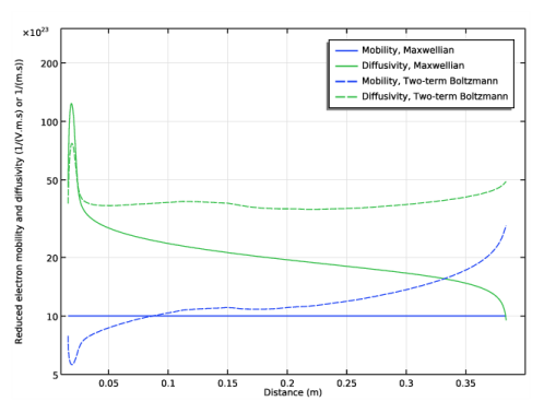
In the Settings window for 1D Plot Group, type Electron Mobility and Diffusivity in the Label text field.
3
Locate the Data section. From the Time selection list, choose Last.
4
Locate the Title section. From the Title type list, choose None.
5
Locate the Plot Settings section. Select the x-axis label check box.
6
7
Select the y-axis label check box.
8
In the associated text field, type Reduced electron mobility and diffusivity (1/(V.m.s) or 1/(m.s)).
9
Locate the Axis section. Select the y-axis log scale check box.
10
Select the Manual axis limits check box.
11
In the x minimum text field, type 0.01.
12
In the x maximum text field, type 0.4.
13
In the y minimum text field, type 5e23.
14
In the y maximum text field, type 3e25.
Line Graph 1
1
Right-click Electron Mobility and Diffusivity and choose Line Graph.
2
In the Settings window for Line Graph, locate the Selection section.
3
From the Selection list, choose All domains.
4
Locate the y-Axis Data section. In the Expression text field, type plas.muexx*plas.Nn.
5
Locate the x-Axis Data section. From the Parameter list, choose Expression.
6
In the Expression text field, type x.
7
Locate the Legends section. Select the Show legends check box.
8
From the Legends list, choose Manual.
9
10
In the Electron Mobility and Diffusivity toolbar, click  Plot.
Line Graph 2
1
Right-click Line Graph 1 and choose Duplicate.
2
In the Settings window for Line Graph, locate the y-Axis Data section.
3
In the Expression text field, type plas.Dexx*plas.Nn.
4
Locate the Legends section. In the table, enter the following settings:
Line Graph 3
1
In the Model Builder window, under Results>Electron Mobility and Diffusivity right-click Line Graph 1 and choose Duplicate.
2
In the Settings window for Line Graph, locate the Data section.
3
From the Dataset list, choose Computed EEDF/Solution 3 (sol3).
4
From the Time selection list, choose Last.
5
Locate the Legends section. In the table, enter the following settings:
6
Locate the Coloring and Style section. From the Color list, choose Cycle (reset).
7
Find the Line style subsection. From the Line list, choose Dashed.
Line Graph 4
1
In the Model Builder window, under Results>Electron Mobility and Diffusivity right-click Line Graph 2 and choose Duplicate.
2
In the Settings window for Line Graph, locate the Data section.
3
From the Dataset list, choose Computed EEDF/Solution 3 (sol3).
4
From the Time selection list, choose Last.
5
Locate the Coloring and Style section. Find the Line style subsection. From the Line list, choose Dashed.
6
Locate the Legends section. In the table, enter the following settings:
7
In the Electron Mobility and Diffusivity toolbar, click  Plot.
Results
Electron Mobility and Diffusivity
In the Model Builder window, collapse the Results>Electron Mobility and Diffusivity node.
Computed EEDF/Solution 3 (5) (sol3)
1
In the Model Builder window, expand the Results>Datasets node.
2
Right-click Results>Datasets>Computed EEDF/Solution 3 (sol3) and choose Duplicate.
3
In the Settings window for Solution, locate the Solution section.
4
From the Component list, choose Extra Dimension from Plasma (plas_eedf_xdim).
Results
In the Model Builder window, collapse the Results>Datasets node.
Electron Energy Distribution Function
1
In the Home toolbar, click  Add Plot Group and choose 1D Plot Group.
2
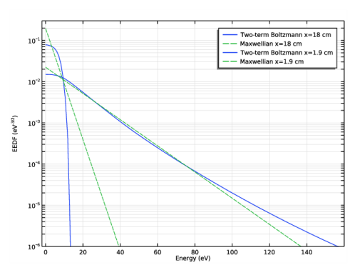
In the Settings window for 1D Plot Group, type Electron Energy Distribution Function in the Label text field.
3
Locate the Data section. From the Dataset list, choose Computed EEDF/Solution 3 (5) (sol3).
4
From the Time selection list, choose Last.
5
Locate the Title section. From the Title type list, choose None.
6
Locate the Plot Settings section. Select the x-axis label check box.
7
8
Select the y-axis label check box.
9
In the associated text field, type EEDF (eV<sup>-3/2</sup>).
10
Locate the Axis section. Select the y-axis log scale check box.
11
Select the Manual axis limits check box.
12
In the x minimum text field, type -2.
13
In the x maximum text field, type 160.
14
In the y minimum text field, type 1e-6.
15
In the y maximum text field, type 0.3.
Line Graph 1
1
Right-click Electron Energy Distribution Function and choose Line Graph.
2
In the Settings window for Line Graph, locate the Selection section.
3
From the Selection list, choose All domains.
4
Locate the y-Axis Data section. In the Expression text field, type atxd1(plas.rcx,plas.fcap).
5
Locate the x-Axis Data section. From the Parameter list, choose Expression.
6
In the Expression text field, type atxd1(plas.rcx,plas.xeedf).
7
Locate the Legends section. Select the Show legends check box.
8
From the Legends list, choose Manual.
9
Line Graph 2
1
Right-click Line Graph 1 and choose Duplicate.
2
In the Settings window for Line Graph, locate the y-Axis Data section.
3
In the Expression text field, type atxd1(plas.rcx,plas.fmax).
4
Locate the Coloring and Style section. Find the Line style subsection. From the Line list, choose Dashed.
5
Locate the Legends section. In the table, enter the following settings:
6
In the Electron Energy Distribution Function toolbar, click  Plot.
Line Graph 3
1
In the Model Builder window, under Results>Electron Energy Distribution Function right-click Line Graph 1 and choose Duplicate.
2
In the Settings window for Line Graph, locate the y-Axis Data section.
3
In the Expression text field, type atxd1(0.019,plas.fcap).
4
Locate the x-Axis Data section. In the Expression text field, type atxd1(0.019,plas.xeedf).
5
Locate the Coloring and Style section. From the Color list, choose Cycle (reset).
6
Locate the Legends section. In the table, enter the following settings:
Line Graph 4
1
In the Model Builder window, under Results>Electron Energy Distribution Function right-click Line Graph 2 and choose Duplicate.
2
In the Settings window for Line Graph, locate the y-Axis Data section.
3
In the Expression text field, type atxd1(0.019,plas.fmax).
4
Locate the x-Axis Data section. In the Expression text field, type atxd1(0.019,plas.xeedf).
5
Locate the Legends section. In the table, enter the following settings:
Results
Electron Energy Distribution Function
1
In the Model Builder window, collapse the Results>Electron Energy Distribution Function node.
2
In the Model Builder window, click Electron Energy Distribution Function.
3
In the Electron Energy Distribution Function toolbar, click  Plot.