|
|
|


|
|
|||
|
1
|
|
2
|
|
3
|
Click Add.
|
|
4
|
Click
|
|
5
|
|
6
|
Click
|
|
1
|
|
2
|
|
1
|
|
2
|
|
1
|
In the Model Builder window, under Component 1 (comp1) right-click Plasma (plas) and choose Global>Cross Section Import.
|
|
2
|
|
3
|
Click Browse.
|
|
5
|
Click Import.
|
|
6
|
|
7
|
|
8
|
|
9
|
Click to expand the Discretization section. From the Formulation list, choose Finite element, log formulation (quadratic shape function).
|
|
1
|
|
2
|
|
3
|
|
4
|
|
1
|
|
2
|
|
3
|
|
4
|
Locate the Reaction Parameters section. From the Rate constant form list, choose Townsend coefficient.
|
|
5
|
|
1
|
|
2
|
|
3
|
|
4
|
Locate the Reaction Parameters section. From the Rate constant form list, choose Townsend coefficient.
|
|
5
|
|
1
|
|
2
|
|
3
|
|
4
|
|
1
|
|
2
|
|
3
|
|
4
|
|
1
|
|
2
|
|
3
|
|
4
|
|
1
|
|
2
|
|
3
|
|
1
|
|
2
|
|
3
|
|
4
|
|
1
|
|
2
|
|
3
|
|
5
|
|
6
|
|
1
|
|
2
|
|
3
|
|
1
|
|
2
|
|
3
|
|
4
|
Click in the Graphics window and then press Ctrl+A to select both boundaries.
|
|
1
|
|
2
|
Click in the Graphics window and then press Ctrl+A to select both boundaries.
|
|
1
|
|
1
|
|
3
|
|
4
|
|
5
|
|
6
|
|
1
|
|
2
|
|
3
|
|
4
|
|
5
|
|
6
|
|
7
|
|
8
|
|
1
|
|
2
|
|
3
|
|
4
|
Click
|
|
5
|
|
6
|
|
7
|
|
8
|
|
9
|
|
10
|
Click Add.
|
|
11
|
|
1
|
|
2
|
|
3
|
|
4
|
In the associated text field, type Distance (m).
|
|
5
|
|
6
|
|
1
|
|
2
|
|
3
|
|
4
|
|
5
|
In the associated text field, type Distance (m).
|
|
6
|
|
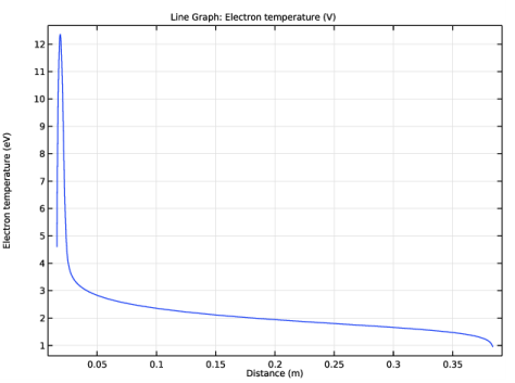
7
|
In the associated text field, type Electron temperature (eV).
|
|
8
|
|
1
|
|
2
|
|
3
|
|
4
|
|
5
|
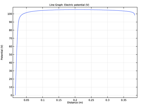
In the associated text field, type Distance (m).
|
|
6
|
|
7
|
In the associated text field, type Potential (V).
|
|
8
|
|
1
|
|
2
|
|
3
|
|
4
|
|
5
|
In the associated text field, type Distance (m).
|
|
6
|
|
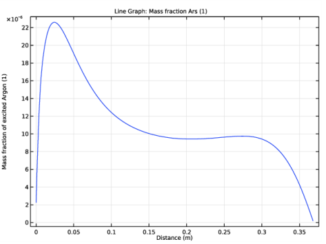
7
|
In the associated text field, type Mass fraction of excited Argon (1).
|
|
1
|
|
3
|
In the Settings window for Line Graph, click Replace Expression in the upper-right corner of the y-Axis Data section. From the menu, choose Component 1 (comp1)>Plasma>Mass fractions>plas.wArs - Mass fraction.
|
|
4
|
|
1
|
|
2
|
|
3
|
|
4
|
|
5
|
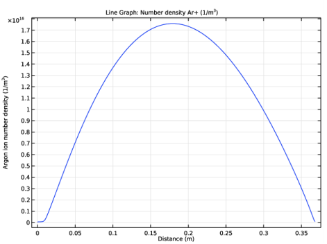
In the associated text field, type Distance (m).
|
|
6
|
|
7
|
In the associated text field, type Argon ion number density (1/m<sup>3</sup>).
|
|
1
|
|
3
|
In the Settings window for Line Graph, click Replace Expression in the upper-right corner of the y-Axis Data section. From the menu, choose Component 1 (comp1)>Plasma>Number densities>plas.n_wAr_1p - Number density - 1/m³.
|
|
4
|
|
1
|
|
2
|
|
3
|
|
4
|
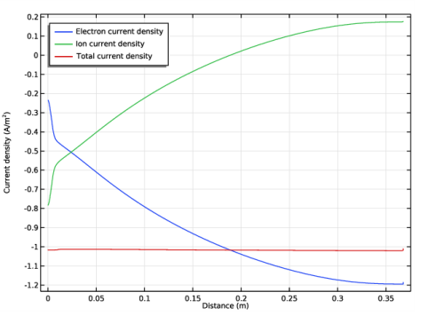
Locate the Plot Settings section. In the y-axis label text field, type Current density (A/m<sup>2</sup>).
|
|
5
|
|
1
|
|
2
|
In the Settings window for Line Graph, click Replace Expression in the upper-right corner of the y-Axis Data section. From the menu, choose Component 1 (comp1)>Plasma>Current>Electron current density - A/m²>plas.Jelx - Electron current density, x component.
|
|
3
|
|
4
|
|
5
|
|
6
|
|
7
|
|
1
|
|
2
|
In the Settings window for Line Graph, click Replace Expression in the upper-right corner of the y-Axis Data section. From the menu, choose Component 1 (comp1)>Plasma>Species>Species wAr_1p>Ion current density - A/m²>plas.Jix_wAr_1p - Ion current density, x component.
|
|
3
|
|
4
|
Locate the Legends section. In the table, enter the following settings:
|
|
1
|
|
2
|
|
3
|
|
4
|
Locate the Legends section. In the table, enter the following settings:
|
|
5
|