Convection Cooling of Circuit Boards

Convection Cooling of Circuit Boards — 3D Forced Convection

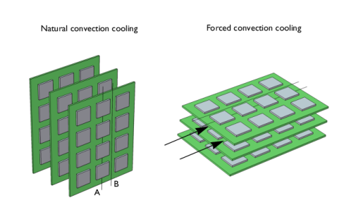
This example models the air cooling of circuit boards populated with multiple integrated circuits (ICs), which act as heat sources. Two possible cooling scenarios are shown in Figure 1: vertically aligned boards using natural convection, and horizontal boards with forced convection (fan cooling). In this case, contributions caused by the induced (forced) flow of air dominate the cooling. To achieve high accuracy, the simulation models heat transport in combination with the fluid flow.

Figure 1: Stacked circuit boards with multiple in-line heat sources. Line A represents the centerline of the row of ICs, and the area between lines A-B on the board represents the symmetry.

A common technique is to describe convective heat flux with a film-resistance coefficient, h. The heat-transfer equations then become simple to solve. However, this simplification requires that the coefficient is well determined which is difficult for many systems and conditions.

An alternative way to thoroughly describe the convective heat transfer is to model the heat transfer in combination with the fluid-flow field. The results then accurately describe the heat transport and temperature changes. From such simulations it is also possible to derive accurate estimations of the film coefficients. Such models are somewhat more complex but they are useful for unusual geometries and complex flows. The following example models the heat transfer of a circuit-board assembly using the Heat Transfer Module’s Conjugate Heat Transfer predefined multiphysics coupling. The modeled scenario is based on work published by A. Ortega (Ref. 1).

FR4 circuit board material (Ref. 2) and silicon are used as the solid materials composing the circuit board system. The model treats air properties as temperature dependent.

The dimensions of the original geometry are:

•

Board: length (in the flow direction) 130 mm, and the thickness is 2 mm

•

ICs: length and width are both 20 mm, and thickness is 2 mm

•

The distance of air between the boards is 10 mm

Model Definition

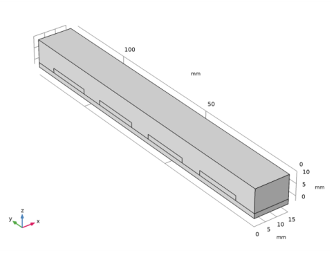
This example simulates the horizontal board with forced convection cooling as shown on the right side of the Figure 1. Due to symmetry, it is sufficient to model a unit cell, from the back side of a board to the next back side, covering the area between lines A and B. Figure 2 depicts the three-dimensional geometry.

Figure 2: The modeled geometries in 3D.

The model makes use of the Conjugate Heat Transfer predefined multiphysics coupling with a stationary study to set up the simulation. The heat rate per unit volume is 1.25 MW/m3. To model forced convection, set up an inlet-velocity profile, uy, that is uniform in the (horizontal) x direction and parabolic (similar to a fully developed laminar profile) in the (vertical) z direction. In terms of an equation this reads

where z = z ⁄(10 mm) parameterizes the height above the board and umax, the maximal inlet speed, equals 1 m/s. At the outlet all the models use the normal flow, zero pressure boundary condition. In addition, no slip conditions at the surfaces of the board and the ICs are applied. You should also set the lateral boundaries periodic with respect to temperature, making the temperatures equal on both boundaries at every y value. Finally, the models apply continuity of temperature and heat flux at all interior boundaries.

Results and Discussion

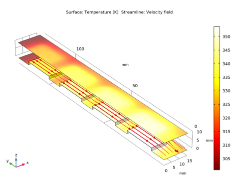
In this example, a forced fluid inlet velocity represents the situation when a fan cools the ICs. Figure 3 shows the resulting temperature distribution. The temperature rise in the ICs is approximately 20–35 K smaller compared to that for natural-convection case (see Convection Cooling of Circuit Boards — 3D Natural Convection for the model description and results). This is due to the higher average fluid velocity. In the forced convection case, the temperature difference along the board is also less pronounced than for the natural convection.

Figure 3: Temperature distribution in the case of forced convection cooling of horizontal boards.

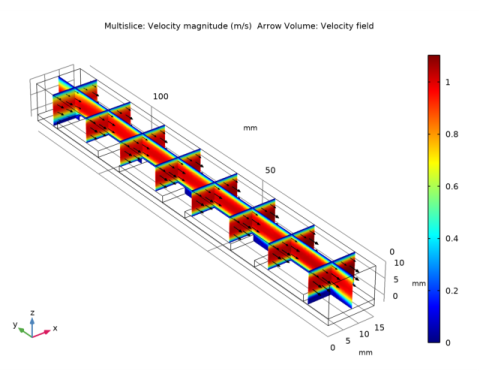
Another interesting result, visible in Figure 4, is that the channeling effect of the gap causes a reduction in the fluid’s flow rate above the sources. The cooling of the ICs is therefore somewhat reduced compared to an ideal case with an even flow field.

Figure 4: Velocity distribution for the case of forced convection.

The symmetry conditions used in the model indicate that the model accounts for multiple chips and boards corresponding to the boards configuration shown in Figure 1. Figure 5 shows the temperature profile on the stacked circuit boards and the streamlines in the surrounding air.

Figure 5: Temperature profile on the stacked circuit boards and streamlines.

References

1. A. Ortega, “Air Cooling of Electronics: A Personal Perspective 1981-2001,” presentation material, IEEE SMITHERM Symposium, 2002.

2. C. Bailey, “Modeling the Effect of Temperature on Product Reliability,” Proc. 19th IEEE SMITHERM Symposium, 2003.

Heat_Transfer_Module/Power_Electronics_and_Electronic_Cooling/circuit_board_forced_3d

Modeling Instructions

From the menu, choose .

New

In the window, click

Model Wizard

In the window, click

In the tree, select .

Click .

Click

In the tree, select .

Click

Global Definitions

Parameters 1

In the window, under click .

In the window for , locate the section.

In the table, enter the following settings:


Name	Expression	Value	Description
q_source	1[W]/(20202[mm^3])	1.25E6 W/m³	Heating power per unit volume
T0	300[K]	300 K	External air temperature
patm	1[atm]	1.0133E5 Pa	Air pressure
umax	1[m/s]	1 m/s	Inlet velocity