PDF

Loudspeaker Driver in a Vented Enclosure
Introduction
This example models the acoustic behavior of a loudspeaker driver mounted in a bass reflex enclosure. The enclosure, sometimes called the cabinet, alters substantially the sensitivity and radiation characteristics of the loudspeaker and it is why it is usually considered part of the integral design of a loudspeaker system.
Two of the most important design parameters for a loudspeaker driver is its sensitivity and the directivity of the system. The sensitivity is commonly defined as the on-axis sound pressure level, measured at a 1 m distance, as the driver is loaded by an AC voltage of 1 W. The directivity is assessed using the Directivity plot and represents the spatial sensitivity plotted against the frequency in a contour-like plot.
To isolate the driver’s performance from that of the environment it usually operates in, the driver is often set directly in an infinite baffle. This approach is used in another example Loudspeaker Driver — Frequency-Domain Analysis model in the Acoustics Module Application Library. The model described here uses the lumped electromagnetic results from that example and shows how the enclosure affects the response of the loudspeaker.
The model represents the structural components through the Solid Mechanics and the Shell physics applied to the different parts of the loudspeaker (enclosure and driver). The acoustic cavity within the enclosure is modeled with the Pressure Acoustics, Frequency Domain physics, while the infinite domain surrounding the enclosure, is modeled with the Pressure Acoustics, Boundary Elements physics. The Acoustic-Structure Boundary multiphysics coupling is used to connect the different acoustic and structural physics and the Acoustic BEM-FEM Boundary multiphysics coupling is use to couple the interior acoustics to the exterior at the vent.
Note: The model requires the Acoustics Module and the Structural Mechanics Module since it involves the use of the Shell interface.
Model Definition
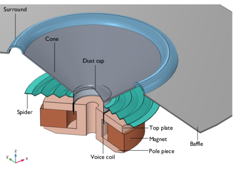
Figure 1 shows the geometry of the considered driver in an infinite baffle, as modeled in the Loudspeaker Driver — Frequency-Domain Analysis example. In the model described here, the driver is set in a frame and placed in a bass reflex enclosure (Figure 2). The defining feature of this enclosure type is the vent, which in a properly designed enclosure acts to boost the sound at low frequencies.
Figure 3 shows the driver mounted in the enclosure. The moving parts of the driver are, in the geometry of this model, represented as surfaces rather than thin volumes. This lets you model them as shells, which vastly reduces the number of mesh elements required to resolve the model. Figure 4 displays the complete model geometry; the interior domain, the driver, and the cabinet. The model uses one symmetry in the xz-plane. The exterior acoustics are modeled with BEM and only require definition on the exterior boundary of the speaker.
Figure 1: The driver, here set in an infinite baffle as in the loudspeaker driver model.
Figure 2: The basket (left )and the vented enclosure with basket and vent (right).
Figure 3: The geometry of the loudspeaker. The enclosure is placed in an anechoic environment (infinite space). The figure also shows the displacements of the structure at 1400 Hz.
Figure 4: The complete model geometry, symmetry with respect to the xz-plane is used.
The model is driven by a lumped representation of the electromagnetic force acting on the voice coil:
The expression is derived in the documentation for the Loudspeaker Driver — Frequency-Domain Analysis model. BL is the so-called force factor of the voice coil and Zb is its blocked coil impedance; the electric impedance as measured/simulated when the coil is at stand-still. BL is a constant 10.48 N/A and Zb is a complex-valued function of the frequency. Both BL and Zb are taken directly from Loudspeaker Driver — Frequency-Domain Analysis, the latter through an interpolation function from a .txt files with the resistive and inductive contributions listed versus the frequency.
V0 is the applied driving voltage. The definition of sensitivity assumes a driving power that equals 1 W when the total impedance of the loudspeaker is at its nominal value. The modeled driver has a nominal impedance of 6.3 Ω, which translates to a driving voltage of = V0eiωt with the amplitude V0 = 3.55 V (peak voltage). The second term in the expression for the driving force contains the axial velocity of the voice coil v, which is unknown prior to the computation.
The electromagnetic force is applied as opposing forces acting over the voice coil and the permanent magnets in opposite directions. As the cone and the suspension move and deform, their local normal acceleration acts as an acoustic source, while the computed acoustic pressure acts back as a load on the shell and solid. This fully coupled behavior is automatically handled by the Acoustic-Structure Boundary multiphysics coupling.
For a discussion of the material and damping parameters used in the moving parts of the driver, see the Loudspeaker Driver — Frequency-Domain Analysis model documentation.
Results and Discussion
The opposing electromagnetic forces create stresses and strains in all the structural parts, as well as a sound pressure distribution inside and outside the enclosure at all frequencies solved for. As an example of how you can visualize the deformations, Figure 3 includes them as a deformed surface plot. Figure 5 shows the acoustic pressure distribution on the surfaces of the enclosure and as a slice plot of a portion of the exterior infinite domain.
Figure 5: Acoustic pressure at 3550 Hz.
Even though the Pressure Acoustics, Boundary Elements physics is only solved for on the boundaries, it is possible to postprocess the solution at any spatial point, as shown in Figure 5 and Figure 6. This makes it possible to, for instance, create slice plots like these two figures or plot the sound pressure level at a given distance versus the elevation angle, or evaluate the directivity as shown in Figure 7.
An alternative option is shown in Figure 6, where the sound pressure level in dB is plotted. Note that the deformation of the cone at this frequency indicates a cone breakup, as discussed in Loudspeaker Driver — Frequency-Domain Analysis.
Figure 6: Sound pressure level at 3550 Hz
Although it is possible to analyze the performance of the loudspeaker by looping through the different pressure plots, a directivity plot can give a good insight into the general performance of the speaker by analyzing some of the features in it. The response of the speaker is evaluated on a circle 1 m around of the speaker, the data is collected for all frequencies and plotted in this contour-like plot. The plot is predefined in the Acoustics Module and is simply called Directivity. Figure 7 shows the directivity plot evaluated for a circles of 1 m radius over the xy-plane (horizontal directivity) and the xz-plane (vertical directivity), respectively.
Figure 7: Directivity of the speaker in the xy-plane (top) and xz-plane (bottom).
These plots reveal that analyzing the loudspeaker in an actual flexible speaker enclosure significantly modifies the directivity characteristics of the loudspeaker. The usual light bulb to flashlight transition appears at a much lower frequency compared to the Loudspeaker Driver — Frequency-Domain Analysis model.
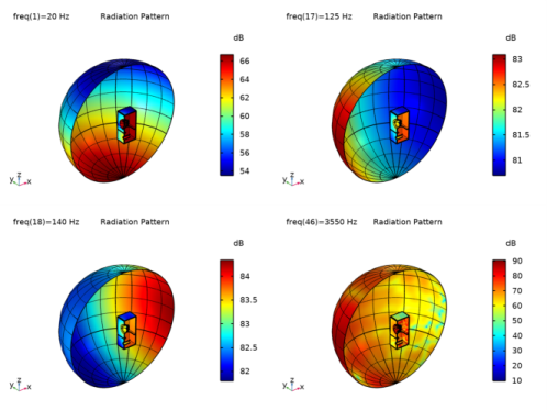
The directivity plot in both planes shows a vertical feature around 140 Hz, which indicates that the loudspeaker is radiating in every direction due to a structural mode of the enclosure. The vertical directivity indicates a high directional behavior (vertical dipole) at very low frequencies, which becomes negligible at around 50 Hz. The radiation pattern features can be seen in detail in Figure 8. The plot is also sometimes known as a bubble plot. Beaming behavior can be observed as the frequency increases.
Figure 8: Radiation patterns at 20 Hz, 125 Hz 140 Hz and 3550 Hz.
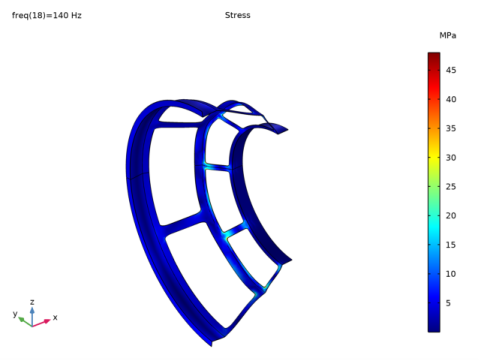
The radiation pattern at 140 Hz, shown in figure Figure 8, shows that the loudspeaker is radiating more to the back than the front of the speaker, which is quite atypical and indicates the presence of an enclosure structural mode. This mode can also be seen in the mode shape plot in Figure 10, and can also be identified by the stress plot in Figure 9, showing significant stresses in the basket of the loudspeaker. At frequencies close to structural modes, the stress results are completely controlled by the damping of the structural components, so small changes in the isotropic loss factor can, in the end, mean a large difference in the stress prediction..
Figure 9: Stress distribution at 140 Hz on the basket.
Figure 10 shows how, as the frequency increases, structural modes with shorter wavelengths become excited. These structural modes, studied in detail in Loudspeaker Driver — Frequency-Domain Analysis, generate a difference in phase of different parts of the cone which reduce the efficiency of the acoustic radiation of the cone.
Figure 10: Displacement at 50 Hz, 1600 Hz 1800 Hz and 3550 Hz
The sensitivity of the speaker system is depicted in Figure 11, when the model us solved with a 1/6 octave frequency resolution (the resolution can be increased in the model if necessary). Compared to the sensitivity of the baffled driver alone (Figure 8 in the Loudspeaker Driver — Frequency-Domain Analysis model), adding the enclosure clearly results in a “boost” for all the frequencies. The addition of flexible components around the loudspeaker produces a complex sensitivity response, caused by the many structural and acoustic modes present. Acoustic features are also visible, like the increased sensitivity around 28 Hz which is due to the interaction of the vent and the loudspeaker cone. The peak at around 65 Hz is caused by the acoustic mode or Helmholtz resonance of the enclosure cavity.
Figure 11: Loudspeaker sensitivity measured as the on-axis sound pressure level (dB) at a distance of 1 m from the unit. The pressure is evaluated using an RMS input signal of 2.51 V, corresponding to a power of 1 W at 6.3 Ω. Note the logarithmic scale for the frequency.
Figure 12: First circumferential mode of the cone (top left), first enclosure mode (top right), first rocking mode of the cone (bottom left), and second enclosure mode (bottom right). These are the main modes influencing the response.
The last study, in the model, is an eigenfrequency analysis considering only the structural components to identify the modes influencing the performance of the speaker.
As seen in Figure 12, a 3D model is able to capture circumferential and rocking cone modes that will not be possible to analyze through an axisymmetric model like Loudspeaker Driver — Frequency-Domain Analysis. The flexible enclosure creates additional structural modes that would not be available if the enclosure was considered as rigid.
Application Library path: Acoustics_Module/Electroacoustic_Transducers/vented_loudspeaker_enclosure
Modeling Instructions
From the File menu, choose New.
New
In the New window, click  Model Wizard.
Model Wizard
1
In the Model Wizard window, click  3D.
2
In the Select Physics tree, select Acoustics>Pressure Acoustics>Pressure Acoustics, Frequency Domain (acpr).
3
Click Add.
4
In the Select Physics tree, select Acoustics>Pressure Acoustics>Pressure Acoustics, Boundary Elements (pabe).
5
Click Add.
6
In the Select Physics tree, select Structural Mechanics>Solid Mechanics (solid).
7
Click Add.
8
In the Select Physics tree, select Structural Mechanics>Shell (shell).
9
Click Add.
10
Click  Study.
11
In the Select Study tree, select General Studies>Frequency Domain.
12
Geometry 1
1
In the Model Builder window, under Component 1 (comp1) click Geometry 1.
2
In the Settings window for Geometry, locate the Units section.
3
From the Length unit list, choose mm.
Import 1 (imp1)
1
In the Home toolbar, click  Import.
2
In the Settings window for Import, locate the Import section.
3
Click Browse.
4
5
Click Import.
Definitions
To make it easier to select some important sets of domains and boundaries in a complicated geometry such as the one you are looking at, it is good modeling practice to begin by defining selections. When working on your own model, these selections are most conveniently defined by clicking and selecting directly in the geometry. The instructions however refer to them by numbers. Whenever a selection is made, it is therefore recommended that you use the Paste Selection button. Enter the number or list of numbers in the text field that appears. Input such as 5, 5-8, 13, or 4, 7, and 9 is accepted.
All Domains
1
In the Model Builder window, expand the Component 1 (comp1)>Definitions node.
2
Right-click Definitions and choose Selections>Explicit.
3
In the Settings window for Explicit, type All Domains in the Label text field.
4
Locate the Input Entities section. Select the All domains check box.
Coil
1
In the Definitions toolbar, click  Explicit.
2
In the Settings window for Explicit, type Coil in the Label text field.
3
Click the  Wireframe Rendering button in the Graphics toolbar.
With wireframe rendering, you can see through boundaries and get a better view of which ones you are selecting.
4
Narrow Region Inner
1
In the Definitions toolbar, click  Explicit.
2
In the Settings window for Explicit, type Narrow Region Inner in the Label text field.
3
Narrow Region Outer
1
In the Definitions toolbar, click  Explicit.
2
In the Settings window for Explicit, type Narrow Region Outer in the Label text field.
3
Soft Iron
1
In the Definitions toolbar, click  Explicit.
2
In the Settings window for Explicit, type Soft Iron in the Label text field.
3
Ferrite
1
In the Definitions toolbar, click  Explicit.
2
In the Settings window for Explicit, type Ferrite in the Label text field.
3
Enclosure
1
In the Definitions toolbar, click  Explicit.
2
In the Settings window for Explicit, type Enclosure in the Label text field.
3
Air Domains
1
In the Definitions toolbar, click  Difference.
2
In the Settings window for Difference, type Air Domains in the Label text field.
3
Locate the Input Entities section. Under Selections to add, click  Add.
4
In the Add dialog box, select All Domains in the Selections to add list.
5
6
In the Settings window for Difference, locate the Input Entities section.
7
Under Selections to subtract, click  Add.
8
In the Add dialog box, in the Selections to subtract list, choose Coil, Soft Iron, Ferrite, and Enclosure.
9
Structural Domains
1
In the Definitions toolbar, click  Union.
2
In the Settings window for Union, type Structural Domains in the Label text field.
3
Locate the Input Entities section. Under Selections to add, click  Add.
4
In the Add dialog box, in the Selections to add list, choose Coil, Soft Iron, Ferrite, and Enclosure.
5
Swept Domains
1
In the Definitions toolbar, click  Union.
2
In the Settings window for Union, type Swept Domains in the Label text field.
3
Locate the Input Entities section. Under Selections to add, click  Add.
4
In the Add dialog box, in the Selections to add list, choose Coil, Narrow Region Inner, Narrow Region Outer, and Enclosure.
5
All Boundaries
1
In the Definitions toolbar, click  Explicit.
2
In the Settings window for Explicit, type All Boundaries in the Label text field.
3
Locate the Input Entities section. From the Geometric entity level list, choose Boundary.
4
Select the All boundaries check box.
Composite
1
In the Definitions toolbar, click  Explicit.
2
In the Settings window for Explicit, type Composite in the Label text field.
3
Locate the Input Entities section. From the Geometric entity level list, choose Boundary.
4
Cloth
1
In the Definitions toolbar, click  Explicit.
2
In the Settings window for Explicit, type Cloth in the Label text field.
3
Locate the Input Entities section. From the Geometric entity level list, choose Boundary.
4
Foam
1
In the Definitions toolbar, click  Explicit.
2
In the Settings window for Explicit, type Foam in the Label text field.
3
Locate the Input Entities section. From the Geometric entity level list, choose Boundary.
4
Glass Fiber
1
In the Definitions toolbar, click  Explicit.
2
In the Settings window for Explicit, type Glass Fiber in the Label text field.
3
Locate the Input Entities section. From the Geometric entity level list, choose Boundary.
4
Basket
1
In the Definitions toolbar, click  Explicit.
2
In the Settings window for Explicit, type Basket in the Label text field.
3
Locate the Input Entities section. From the Geometric entity level list, choose Boundary.
4
Other Mapped Boundaries
1
In the Definitions toolbar, click  Explicit.
2
In the Settings window for Explicit, type Other Mapped Boundaries in the Label text field.
3
Locate the Input Entities section. From the Geometric entity level list, choose Boundary.
4
Not Mapped Boundaries
1
In the Definitions toolbar, click  Explicit.
2
In the Settings window for Explicit, type Not Mapped Boundaries in the Label text field.
3
Locate the Input Entities section. From the Geometric entity level list, choose Boundary.
4
Shell Domains
1
In the Definitions toolbar, click  Union.
2
In the Settings window for Union, type Shell Domains in the Label text field.
3
Locate the Geometric Entity Level section. From the Level list, choose Boundary.
4
Locate the Input Entities section. Under Selections to add, click  Add.
5
In the Add dialog box, in the Selections to add list, choose Composite, Cloth, Foam, Glass Fiber, and Basket.
6
Symmetry Boundaries
1
In the Definitions toolbar, click  Box.
2
In the Settings window for Box, type Symmetry Boundaries in the Label text field.
3
Locate the Geometric Entity Level section. From the Level list, choose Boundary.
4
Locate the Box Limits section. In the y maximum text field, type 0.
5
Locate the Output Entities section. From the Include entity if list, choose Entity inside box.
Boundaries out of Symmetry Plane
1
In the Definitions toolbar, click  Difference.
2
In the Settings window for Difference, type Boundaries out of Symmetry Plane in the Label text field.
3
Locate the Geometric Entity Level section. From the Level list, choose Boundary.
4
Locate the Input Entities section. Under Selections to add, click  Add.
5
In the Add dialog box, select All Boundaries in the Selections to add list.
6
7
In the Settings window for Difference, locate the Input Entities section.
8
Under Selections to subtract, click  Add.
9
In the Add dialog box, select Symmetry Boundaries in the Selections to subtract list.
10
Mapped Boundaries
1
In the Definitions toolbar, click  Difference.
2
In the Settings window for Difference, type Mapped Boundaries in the Label text field.
3
Locate the Geometric Entity Level section. From the Level list, choose Boundary.
4
Locate the Input Entities section. Under Selections to add, click  Add.
5
In the Add dialog box, in the Selections to add list, choose Cloth, Foam, Glass Fiber, and Other Mapped Boundaries.
6
7
In the Settings window for Difference, locate the Input Entities section.
8
Under Selections to subtract, click  Add.
9
In the Add dialog box, select Not Mapped Boundaries in the Selections to subtract list.
10
Symmetry Edges
1
In the Definitions toolbar, click  Box.
2
In the Settings window for Box, type Symmetry Edges in the Label text field.
3
Locate the Geometric Entity Level section. From the Level list, choose Edge.
4
Locate the Box Limits section. In the y maximum text field, type 0.
5
Locate the Output Entities section. From the Include entity if list, choose Entity inside box.
Next, define interpolation functions to bring in the blocked resistance and inductance from the model of the driver.
Interpolation 1 (int1)
1
In the Definitions toolbar, click  Interpolation.
2
In the Settings window for Interpolation, locate the Definition section.
3
From the Data source list, choose File.
4
Click Browse.
5
6
Click Import.
7
In the Function name text field, type Rb.
8
Locate the Units section. In the Arguments text field, type Hz.
9
In the Function text field, type ohm.
Interpolation 2 (int2)
1
In the Definitions toolbar, click  Interpolation.
2
In the Settings window for Interpolation, locate the Definition section.
3
From the Data source list, choose File.
4
Click Browse.
5
6
Click Import.
7
In the Function name text field, type Lb.
8
Locate the Units section. In the Arguments text field, type Hz.
9
In the Function text field, type H.
To enable extraction of the velocity, define an average operator acting on the voice coil.
Average 1 (aveop1)
1
In the Definitions toolbar, click  Nonlocal Couplings and choose Average.
2
In the Settings window for Average, type av_coil in the Operator name text field.
3
Locate the Source Selection section. From the Selection list, choose Coil.
Global Definitions
Define parameters for the driving voltage, the BL factor from the loudspeaker driver model, the frequency at which the material losses are specified, and the wavelength at 3550 Hz (used to set the mesh size).
Parameters 1
1
In the Model Builder window, under Global Definitions click Parameters 1.
2
In the Settings window for Parameters, locate the Parameters section.
3
Definitions
Next, create the expressions used in defining the electric driving force. The Description field is optional, but helps you keep track of what you are doing.
Variables 1
1
In the Definitions toolbar, click  Local Variables.
2
In the Settings window for Variables, locate the Variables section.
3
Materials
While the material properties used in this model are partly made up, they resemble those used in a real driver. The coil former has properties representative of glass fiber materials. The spider, acting as a spring, is made of a phenolic cloth with a much lower stiffness. The material used in the coil is taken to be lighter than copper, as the wire is insulated and does not completely fill the coil domain. The surround, finally, is a light resistive foam.
Except for air and soft Iron, the materials you will use all come from a material library created especially for this model (to be loaded from the file loudspeaker_driver_materials.mph). You may notice that some of the materials will report missing properties. For example, the composite does not include any electromagnetic properties. This is fine, as you will not model the magnetic fields in the domains where the composite is used.
Add Material
1
In the Home toolbar, click  Add Material to open the Add Material window.
2
Go to the Add Material window.
3
4
Click Add to Component in the window toolbar.
5
In the tree, select Built-in>Structural steel.
6
Click Add to Component in the window toolbar.
Add this material twice as it will be used in the Solid and the Shell Physics.
7
In the tree, select Built-in>Structural steel.
8
Click Add to Component in the window toolbar.
Materials
Structural steel 1 (mat3)
Right-click Component 1 (comp1)>Materials>Structural steel 1 (mat3) and choose Browse Materials.
Material Browser
1
In the Material Browser window, In the ribbon make sure to select the Materials tab and then click the Browse Materials icon.
The Import Material Library functionality is activated by clicking the small icon at the lower-right, below the Material Browser tree.
2
click  Import Material Library.
3
4
Add Material
1
Go to the Add Material window.
2
In the tree, select loudspeaker driver materials>Composite.
3
Click Add to Component in the window toolbar.
4
In the tree, select loudspeaker driver materials>Cloth.
5
Click Add to Component in the window toolbar.
6
In the tree, select loudspeaker driver materials>Foam.
7
Click Add to Component in the window toolbar.
8
In the tree, select loudspeaker driver materials>Coil.
9
Click Add to Component in the window toolbar.
10
In the tree, select loudspeaker driver materials>Glass Fiber.
11
Click Add to Component in the window toolbar.
12
In the tree, select loudspeaker driver materials>Generic Ferrite.
13
Click Add to Component in the window toolbar.
14
In the tree, select loudspeaker driver materials>Fiberboard.
15
Click Add to Component in the window toolbar.
16
In the Home toolbar, click  Add Material to close the Add Material window.
Materials
Air (mat1)
1
In the Model Builder window, under Component 1 (comp1)>Materials click Air (mat1).
2
In the Settings window for Material, locate the Geometric Entity Selection section.
3
From the Selection list, choose All domains and voids.
Structural steel (mat2)
1
In the Model Builder window, click Structural steel (mat2).
2
In the Settings window for Material, locate the Geometric Entity Selection section.
3
From the Selection list, choose Soft Iron.
Structural steel 1 (mat3)
1
In the Model Builder window, click Structural steel 1 (mat3).
2
In the Settings window for Material, locate the Geometric Entity Selection section.
3
From the Geometric entity level list, choose Boundary.
4
From the Selection list, choose Basket.
Composite (mat4)
1
In the Model Builder window, click Composite (mat4).
2
In the Settings window for Material, locate the Geometric Entity Selection section.
3
From the Geometric entity level list, choose Boundary.
4
From the Selection list, choose Composite.
Cloth (mat5)
1
In the Model Builder window, click Cloth (mat5).
2
In the Settings window for Material, locate the Geometric Entity Selection section.
3
From the Geometric entity level list, choose Boundary.
4
From the Selection list, choose Cloth.
Foam (mat6)
1
In the Model Builder window, click Foam (mat6).
2
In the Settings window for Material, locate the Geometric Entity Selection section.
3
From the Geometric entity level list, choose Boundary.
4
From the Selection list, choose Foam.
Coil (mat7)
1
In the Model Builder window, click Coil (mat7).
2
In the Settings window for Material, locate the Geometric Entity Selection section.
3
From the Selection list, choose Coil.
Glass Fiber (mat8)
1
In the Model Builder window, click Glass Fiber (mat8).
2
In the Settings window for Material, locate the Geometric Entity Selection section.
3
From the Geometric entity level list, choose Boundary.
4
From the Selection list, choose Glass Fiber.
Generic Ferrite (mat9)
1
In the Model Builder window, click Generic Ferrite (mat9).
2
In the Settings window for Material, locate the Geometric Entity Selection section.
3
From the Selection list, choose Ferrite.
Fiberboard (mat10)
1
In the Model Builder window, click Fiberboard (mat10).
2
In the Settings window for Material, locate the Geometric Entity Selection section.
3
From the Selection list, choose Enclosure.
With the materials defined, it is now time to set up the remaining physics of the model. Begin by specifying the symmetry condition in the acoustics domain.
Pressure Acoustics, Frequency Domain (acpr)
1
In the Model Builder window, under Component 1 (comp1) click Pressure Acoustics, Frequency Domain (acpr).
2
In the Settings window for Pressure Acoustics, Frequency Domain, locate the Domain Selection section.
3
From the Selection list, choose Air Domains.
Symmetry 1
1
In the Physics toolbar, click  Boundaries and choose Symmetry.
2
In the Settings window for Symmetry, locate the Boundary Selection section.
3
From the Selection list, choose Symmetry Boundaries.
Next add the Narrow Region Acoustics features to account for the losses in the domains surrounding the voice coil. The values of the slit heights are taken from the 2D Axisymmetric model and differ from the measurements of the geometry, as the thickness of the coil former is not specifically captured in the geometry.
Narrow Region Acoustics 1
1
In the Physics toolbar, click  Domains and choose Narrow Region Acoustics.
2
In the Settings window for Narrow Region Acoustics, locate the Domain Selection section.
3
From the Selection list, choose Narrow Region Inner.
4
Locate the Duct Properties section. From the Duct type list, choose Slit.
5
In the h text field, type 0.4[mm].
Narrow Region Acoustics 2
1
In the Physics toolbar, click  Domains and choose Narrow Region Acoustics.
2
In the Settings window for Narrow Region Acoustics, locate the Domain Selection section.
3
From the Selection list, choose Narrow Region Outer.
4
Locate the Duct Properties section. From the Duct type list, choose Slit.
5
In the h text field, type 0.2[mm].
The Pressure Acoustics, Boundary Elements physics lets you compute the pressure field (including phase) at any finite distance from the loudspeaker. Specify the symmetry condition of the xz-plane.
Pressure Acoustics, Boundary Elements (pabe)
1
In the Model Builder window, under Component 1 (comp1) click Pressure Acoustics, Boundary Elements (pabe).
2
In the Settings window for Pressure Acoustics, Boundary Elements, locate the Domain Selection section.
3
From the Selection list, choose All voids.
4
Click to expand the Symmetry/Infinite Boundary Condition section. From the Condition for the y = y^0 plane list, choose Symmetric/Infinite sound hard boundary.
Solid Mechanics (solid)
1
In the Model Builder window, under Component 1 (comp1) click Solid Mechanics (solid).
2
In the Settings window for Solid Mechanics, locate the Domain Selection section.
3
From the Selection list, choose Structural Domains.
Symmetry 1
1
In the Physics toolbar, click  Boundaries and choose Symmetry.
2
In the Settings window for Symmetry, locate the Boundary Selection section.
3
From the Selection list, choose Symmetry Boundaries.
Linear Elastic Material 1
In the Model Builder window, click Linear Elastic Material 1.
Damping 1
1
In the Physics toolbar, click  Attributes and choose Damping.
2
In the Settings window for Damping, locate the Damping Settings section.
3
From the Damping type list, choose Isotropic loss factor.
Next, apply the opposing electromagnetic forces acting onto the coil and magnets.
Body Load 1
1
In the Physics toolbar, click  Domains and choose Body Load.
2
In the Settings window for Body Load, locate the Domain Selection section.
3
From the Selection list, choose Soft Iron.
4
Locate the Force section. From the Load type list, choose Total force.
5
Specify the Ftot vector as
Body Load 2
1
In the Physics toolbar, click  Domains and choose Body Load.
2
In the Settings window for Body Load, locate the Domain Selection section.
3
From the Selection list, choose Coil.
4
Locate the Force section. From the Load type list, choose Total force.
5
Specify the Ftot vector as
Now set up the shell physics. Begin by specifying the individual thicknesses and damping properties of the moving parts of the driver.
Shell (shell)
1
In the Model Builder window, under Component 1 (comp1) click Shell (shell).
2
In the Settings window for Shell, locate the Boundary Selection section.
3
From the Selection list, choose Shell Domains.
Linear Elastic Material 1
In the Model Builder window, under Component 1 (comp1)>Shell (shell) click Linear Elastic Material 1.
Damping 1
1
In the Physics toolbar, click  Attributes and choose Damping.
2
In the Settings window for Damping, locate the Boundary Selection section.
3
From the Selection list, choose Shell Domains.
4
Locate the Damping Settings section. From the Damping type list, choose Isotropic loss factor.
Linear Elastic Material 1
In the Model Builder window, click Linear Elastic Material 1.
Damping 2
1
In the Physics toolbar, click  Attributes and choose Damping.
2
In the Settings window for Damping, locate the Boundary Selection section.
3
From the Selection list, choose Cloth.
4
Locate the Damping Settings section. In the βdK text field, type 0.14/omega_loss.
Linear Elastic Material 1
In the Model Builder window, click Linear Elastic Material 1.
Damping 3
1
In the Physics toolbar, click  Attributes and choose Damping.
2
In the Settings window for Damping, locate the Boundary Selection section.
3
From the Selection list, choose Foam.
4
Locate the Damping Settings section. In the βdK text field, type 0.46/omega_loss.
Thickness and Offset 1
Change the thickness in the default node to 1[mm], this will be applied to the Cone of the speaker. Set the thickness of the other speaker parts.
1
In the Model Builder window, click Thickness and Offset 1.
2
In the Settings window for Thickness and Offset, locate the Thickness and Offset section.
3
In the d text field, type 1[mm].
Thickness and Offset 2
1
In the Physics toolbar, click  Boundaries and choose Thickness and Offset.
2
In the Settings window for Thickness and Offset, locate the Boundary Selection section.
3
From the Selection list, choose Cloth.
4
Locate the Thickness and Offset section. In the d text field, type 0.4[mm].
Thickness and Offset 3
1
In the Physics toolbar, click  Boundaries and choose Thickness and Offset.
2
In the Settings window for Thickness and Offset, locate the Boundary Selection section.
3
From the Selection list, choose Foam.
4
Locate the Thickness and Offset section. In the d text field, type 1.5[mm].
Thickness and Offset 4
1
In the Physics toolbar, click  Boundaries and choose Thickness and Offset.
2
In the Settings window for Thickness and Offset, locate the Boundary Selection section.
3
From the Selection list, choose Glass Fiber.
4
Locate the Thickness and Offset section. In the d text field, type 0.2[mm].
Thickness and Offset 5
1
In the Physics toolbar, click  Boundaries and choose Thickness and Offset.
2
In the Settings window for Thickness and Offset, locate the Boundary Selection section.
3
From the Selection list, choose Basket.
4
Locate the Thickness and Offset section. In the d text field, type 0.8[mm].
Next, add a symmetry condition for the edges in the xz-plane.
Symmetry 1
1
In the Physics toolbar, click  Edges and choose Symmetry.
2
In the Settings window for Symmetry, locate the Edge Selection section.
3
From the Selection list, choose Symmetry Edges.
Update the Structural Steel material to add the isotropic structural loss factor of 0.01.
Materials
Structural steel (mat2)
1
In the Model Builder window, under Component 1 (comp1)>Materials click Structural steel (mat2).
2
In the Settings window for Material, locate the Material Contents section.
3
Structural steel 1 (mat3)
1
In the Model Builder window, click Structural steel 1 (mat3).
2
In the Settings window for Material, locate the Material Contents section.
3
In the following steps, add the multiphysics couplings between the different physics.
Multiphysics
Acoustic-Structure Boundary 1 (asb1)
1
In the Physics toolbar, click  Multiphysics Couplings and choose Boundary>Acoustic-Structure Boundary.
2
In the Settings window for Acoustic-Structure Boundary, locate the Boundary Selection section.
3
From the Selection list, choose All boundaries.
Acoustic-Structure Boundary 2 (asb2)
1
In the Physics toolbar, click  Multiphysics Couplings and choose Boundary>Acoustic-Structure Boundary.
2
In the Settings window for Acoustic-Structure Boundary, locate the Boundary Selection section.
3
From the Selection list, choose All boundaries.
4
Locate the Coupled Interfaces section. From the Structure list, choose Shell (shell).
Acoustic-Structure Boundary 3 (asb3)
1
In the Physics toolbar, click  Multiphysics Couplings and choose Boundary>Acoustic-Structure Boundary.
2
In the Settings window for Acoustic-Structure Boundary, locate the Boundary Selection section.
3
From the Selection list, choose Boundaries out of Symmetry Plane.
4
Locate the Coupled Interfaces section. From the Acoustics list, choose Pressure Acoustics, Boundary Elements (pabe).
Acoustic-Structure Boundary 4 (asb4)
1
In the Physics toolbar, click  Multiphysics Couplings and choose Boundary>Acoustic-Structure Boundary.
2
In the Settings window for Acoustic-Structure Boundary, locate the Boundary Selection section.
3
From the Selection list, choose Boundaries out of Symmetry Plane.
4
Locate the Coupled Interfaces section. From the Acoustics list, choose Pressure Acoustics, Boundary Elements (pabe).
5
From the Structure list, choose Shell (shell).
Acoustic BEM-FEM Boundary 1 (aab1)
1
In the Physics toolbar, click  Multiphysics Couplings and choose Boundary>Acoustic BEM-FEM Boundary.
2
Solid-Thin Structure Connection 1 (sshc1)
1
In the Physics toolbar, click  Multiphysics Couplings and choose Global>Solid-Thin Structure Connection.
2
In the Settings window for Solid-Thin Structure Connection, locate the Connection Settings section.
3
From the Connection type list, choose Shared boundaries.
The mesh needs to resolve the fine details of the geometry as well as the waves at all frequencies. It is always recommended to have at least two elements through the thickness of thin structures to accurately capture the bending stiffness.
Mesh 1
Mapped 1
1
In the Mesh toolbar, click  Boundary and choose Mapped.
2
In the Settings window for Mapped, locate the Boundary Selection section.
3
From the Selection list, choose Mapped Boundaries.
Distribution 1
1
Right-click Mapped 1 and choose Distribution.
2
3
In the Settings window for Distribution, locate the Distribution section.
4
In the Number of elements text field, type 2.
Distribution 2
1
In the Model Builder window, right-click Mapped 1 and choose Distribution.
2
3
In the Settings window for Distribution, locate the Distribution section.
4
In the Number of elements text field, type 10.
Size
1
In the Model Builder window, click Size.
2
In the Settings window for Size, locate the Element Size section.
3
Click the Custom button.
4
Locate the Element Size Parameters section. In the Maximum element size text field, type lam0/4.
5
In the Minimum element size text field, type 2[mm].
This gives you a minimum of 4 elements per wavelength at the highest frequency, 3550 Hz. In practice, remember that a mesh convergence analysis is always recommended.
The shortest edges of the geometry have length 1 mm, which you will resolve with this setting. You can increase the Minimum element size setting to get a coarser mesh in the narrow region. This can trigger a warning as COMSOL checks if the minimum size is larger than a geometric entity. The model will solve when a warning is present. It is up to the user to decide if the warning is relevant for the quality of the simulation results.
Use a swept mesh for some of the domains, this will reduce the running time of the model.
Swept 1
1
In the Mesh toolbar, click  Swept.
2
In the Settings window for Swept, locate the Domain Selection section.
3
From the Geometric entity level list, choose Domain.
4
From the Selection list, choose Swept Domains.
Distribution 1
1
Right-click Swept 1 and choose Distribution.
2
3
In the Settings window for Distribution, locate the Distribution section.
4
In the Number of elements text field, type 2.
Free Tetrahedral 1
1
In the Mesh toolbar, click  Free Tetrahedral.
2
In the Settings window for Free Tetrahedral, click to expand the Element Quality Optimization section.
3
From the Optimization level list, choose High.
This option increases the level of optimization of the meshing operation, which will increase the quality of the mesh while slightly increasing the time required for the meshing operation.
Size 1
1
Right-click Free Tetrahedral 1 and choose Size.
2
In the Settings window for Size, locate the Geometric Entity Selection section.
3
From the Geometric entity level list, choose Boundary.
4
From the Selection list, choose Composite.
5
Locate the Element Size section. Click the Custom button.
6
Locate the Element Size Parameters section. Select the Maximum element size check box.
7
8
Click  Build All.
The plot should look like this.
Study 1 - Complete Study
1
In the Model Builder window, click Study 1.
2
In the Settings window for Study, type Study 1 - Complete Study in the Label text field.
3
Locate the Study Settings section. Clear the Generate default plots check box.
Step 1: Frequency Domain
1
In the Model Builder window, under Study 1 - Complete Study click Step 1: Frequency Domain.
2
In the Settings window for Frequency Domain, locate the Study Settings section.
3
Click  Range.
4
In the Range dialog box, choose ISO preferred frequencies from the Entry method list.
5
In the Start frequency text field, type 20.
6
In the Stop frequency text field, type 3550.
7
From the Interval list, choose 1/6 octave.
8
Click Replace.
9
In the Settings window for Frequency Domain, locate the Study Settings section.
10
From the Reuse solution from previous step list, choose No.
This gives you frequencies with a 1/6 octave resolution from 20 to 3550 Hz with values specified by the ISO standard. The model takes about 30 GB of RAM to solve and will solve in around 90 min (depending on your hardware). If you are short on time you can, for example, select 1/3 octave or simply octave spacing.
11
Right-click Study 1 - Complete Study>Step 1: Frequency Domain and choose Get Initial Value for Step.
Getting the initial values of the step creates also the solver suggestions based on the existing physics. We will use the direct solver suggestion in this model. In the current setup of the model using a direct solver is faster than the default iterative. Here the BEM problem is small compared to the FEM part. If an iterative solver is used, then note that efficient convergence at the higher frequencies will require the use of the Stabilized BEM formulation.
Solver Configurations
In the Model Builder window, expand the Study 1 - Complete Study>Solver Configurations node.
Solution 1 (sol1)
1
In the Model Builder window, expand the Study 1 - Complete Study>Solver Configurations>Solution 1 (sol1)>Stationary Solver 1 node.
2
Right-click Suggested Direct Solver (aab1_asb4_asb1_sshc1_asb3_asb2) and choose Enable.
3
In the Home toolbar, click  Compute.
Now that the model has been solved, proceed to generate the plots.
Results
In the Model Builder window, expand the Results node.
Grid 3D 1
1
In the Model Builder window, expand the Results>Datasets node.
2
Right-click Results>Datasets and choose More 3D Datasets>Grid 3D.
This dataset allows for the evaluation of the boundary elements solution at any spatial location in the model.
3
In the Settings window for Grid 3D, locate the Parameter Bounds section.
4
Find the First parameter subsection. In the Minimum text field, type -500[mm].
5
In the Maximum text field, type 500[mm].
6
Find the Second parameter subsection. In the Minimum text field, type 0.1[mm].
7
In the Maximum text field, type 500[mm].
8
Find the Third parameter subsection. In the Minimum text field, type -400[mm].
9
In the Maximum text field, type 300[mm].
These coordinates define a box surrounding the speaker where we will plot the variables.
10
Click to expand the Resolution section. In the x resolution text field, type 100.
11
In the y resolution text field, type 100.
12
In the z resolution text field, type 100.
Increase the resolution from the default values. This produces smoother plots but may increase the time required for evaluating the solution in a plot.
13
The plot should look like this.
Acoustic Pressure
1
In the Results toolbar, click  3D Plot Group.
2
In the Settings window for 3D Plot Group, type Acoustic Pressure in the Label text field.
3
Click to expand the Title section. From the Title type list, choose Label.
4
Locate the Plot Settings section. Clear the Plot dataset edges check box.
5
Locate the Color Legend section. Select the Show units check box.
Surface 1
1
Right-click Acoustic Pressure and choose Surface.
2
In the Settings window for Surface, locate the Expression section.
3
In the Expression text field, type if(isnan(acpr.p_t),pabe.p_t_bnd,acpr.p_t).
This will plot the total acoustic pressure for both acoustic physics defined in the model.
4
Locate the Coloring and Style section. From the Color table list, choose Wave.
5
Select the Symmetrize color range check box.
Deformation 1
1
Right-click Surface 1 and choose Deformation.
2
In the Settings window for Deformation, locate the Expression section.
3
In the X component text field, type if(isnan(shell.disp),u,u2).
4
In the Y component text field, type if(isnan(shell.disp),v,v2).
5
In the Z component text field, type if(isnan(shell.disp),w,w2).
This is the displacement of the structure obtained from the shell or the solid interface.
Line 1
1
In the Model Builder window, right-click Acoustic Pressure and choose Line.
2
In the Settings window for Line, locate the Expression section.
3
In the Expression text field, type 0.
4
Locate the Coloring and Style section. From the Coloring list, choose Uniform.
5
From the Color list, choose Black.
6
Click to expand the Inherit Style section. From the Plot list, choose Surface 1.
7
Clear the Color check box.
8
Clear the Color and data range check box.
9
Clear the Height scale factor check box.
10
Clear the Tube radius scale factor check box.
Deformation 1
In the Model Builder window, right-click Deformation 1 and choose Copy.
Deformation 1
In the Model Builder window, right-click Line 1 and choose Paste Deformation.
Multislice 1
1
In the Acoustic Pressure toolbar, click  More Plots and choose Multislice.
2
In the Settings window for Multislice, locate the Data section.
3
From the Dataset list, choose Grid 3D 1.
4
Locate the Expression section. In the Expression text field, type pabe.p_t.
5
Locate the Multiplane Data section. Find the x-planes subsection. From the Entry method list, choose Coordinates.
6
In the Coordinates text field, type 125[mm].
7
Find the z-planes subsection. From the Entry method list, choose Coordinates.
8
In the Coordinates text field, type 0.
9
Click to expand the Inherit Style section. From the Plot list, choose Surface 1.
10
Click the  Show Grid button in the Graphics toolbar.
11
In the Acoustic Pressure toolbar, click  Plot.
The result should look like Figure 5.
Sound Pressure Level
1
In the Model Builder window, right-click Acoustic Pressure and choose Duplicate.
2
In the Model Builder window, click Acoustic Pressure 1.
3
In the Settings window for 3D Plot Group, type Sound Pressure Level in the Label text field.
Surface 1
1
In the Model Builder window, click Surface 1.
2
In the Settings window for Surface, locate the Expression section.
3
In the Expression text field, type if(isnan(acpr.Lp),pabe.Lp_bnd,acpr.Lp).
4
Locate the Coloring and Style section. From the Color table list, choose Rainbow.
5
Clear the Symmetrize color range check box.
6
Click to expand the Quality section. From the Resolution list, choose Extra fine.
Multislice 1
1
In the Model Builder window, click Multislice 1.
2
In the Settings window for Multislice, locate the Expression section.
3
In the Expression text field, type pabe.Lp.
4
In the Sound Pressure Level toolbar, click  Plot.
The result should look like Figure 6.
Displacement
1
In the Model Builder window, right-click Sound Pressure Level and choose Duplicate.
2
In the Model Builder window, click Sound Pressure Level 1.
3
In the Settings window for 3D Plot Group, type Displacement in the Label text field.
Surface 1
1
In the Model Builder window, click Surface 1.
2
In the Settings window for Surface, locate the Expression section.
3
In the Expression text field, type if(isnan(shell.disp),solid.disp,shell.disp).
Multislice 1
In the Model Builder window, right-click Multislice 1 and choose Delete.
Displacement
1
In the Model Builder window, click Displacement.
2
In the Displacement toolbar, click  Plot.
Loop through the frequencies to reproduce the results in Figure 2 and Figure 10.
Stress
1
Right-click Displacement and choose Duplicate.
2
In the Model Builder window, click Displacement 1.
3
In the Settings window for 3D Plot Group, type Stress in the Label text field.
4
Locate the Data section. From the Parameter value (freq (Hz)) list, choose 140.
In the next steps, a selection is created to show only the stress results at the basket. This selection can be modified or removed completely to analyze other areas of the model.
5
Click to expand the Selection section. From the Geometric entity level list, choose Boundary.
6
From the Selection list, choose Basket.
7
Select the Apply to dataset edges check box.
Surface 1
1
In the Model Builder window, click Surface 1.
2
In the Settings window for Surface, locate the Expression section.
3
In the Expression text field, type if(isnan(shell.mises),solid.mises,shell.mises).
4
From the Unit list, choose MPa.
5
In the Stress toolbar, click  Plot.
The result should look like Figure 9.
Radiation Pattern
1
In the Model Builder window, right-click Sound Pressure Level and choose Duplicate.
2
In the Model Builder window, click Sound Pressure Level 1.
3
In the Settings window for 3D Plot Group, type Radiation Pattern in the Label text field.
Multislice 1
In the Model Builder window, right-click Multislice 1 and choose Delete.
Radiation Pattern
In the Model Builder window, click Radiation Pattern.
Radiation Pattern 1
1
In the Radiation Pattern toolbar, click  More Plots and choose Radiation Pattern.
2
In the Settings window for Radiation Pattern, locate the Expression section.
3
In the Expression text field, type 1000[mm].
4
Clear the Use as color expression check box.
5
Locate the Color section. In the Expression text field, type pabe.Lp.
6
Locate the Evaluation section. Find the Angles subsection. In the Number of elevation angles text field, type 160.
7
In the Number of azimuth angles text field, type 320.
8
From the Restriction list, choose Manual.
9
In the φ range text field, type 180.
10
Find the Sphere subsection. From the Sphere list, choose Manual.
11
In the Radius text field, type 1000[mm].
12
Locate the Coloring and Style section. From the Grid list, choose Fine.
13
In the Radiation Pattern toolbar, click  Plot.
14
Click the  Zoom Extents button in the Graphics toolbar.
Surface 1
1
In the Model Builder window, click Surface 1.
2
In the Settings window for Surface, locate the Coloring and Style section.
3
Clear the Color legend check box.
4
In the Radiation Pattern toolbar, click  Plot.
Loop through the frequencies to reproduce the results in Figure 8.
Sensitivity at 1 m.
1
In the Home toolbar, click  Add Plot Group and choose 1D Plot Group.
2
In the Settings window for 1D Plot Group, type Sensitivity at 1 m. in the Label text field.
3
Click to expand the Title section. From the Title type list, choose Label.
Octave Band 1
1
In the Sensitivity at 1 m. toolbar, click  More Plots and choose Octave Band.
2
In the Settings window for Octave Band, locate the Selection section.
3
From the Geometric entity level list, choose Global.
4
Locate the y-Axis Data section. In the Expression text field, type at3_spatial(-1[m],0,0,pabe.p_t,'minc').
5
Locate the Plot section. From the Style list, choose Continuous.
6
In the Sensitivity at 1 m. toolbar, click  Plot.
The result should look like Figure 11.
Directivity xy-plane
1
In the Home toolbar, click  Add Plot Group and choose 1D Plot Group.
2
In the Settings window for 1D Plot Group, type Directivity xy-plane in the Label text field.
3
Locate the Title section. From the Title type list, choose Label.
Directivity 1
1
In the Directivity xy-plane toolbar, click  More Plots and choose Directivity.
2
In the Settings window for Directivity, locate the Expression section.
3
In the Expression text field, type pabe.Lp_t.
4
Locate the Evaluation section. Find the Angles subsection. In the Number of angles text field, type 180.
5
From the Restriction list, choose Manual.
6
In the φ start text field, type -180.
7
Find the Evaluation distance subsection. In the Radius text field, type 1000[mm].
8
Find the Reference direction subsection. In the x text field, type -1.
9
Locate the Levels section. From the Entry method list, choose Levels.
10
In the Levels text field, type 9 6 3 1.5 -1.5 -3 -6 -9 -12 -18 -24.
11
In the Directivity xy-plane toolbar, click  Plot.
12
Click the  x-Axis Log Scale button in the Graphics toolbar.
The result should look like Figure 7.
Directivity xz-plane
1
In the Model Builder window, right-click Directivity xy-plane and choose Duplicate.
2
In the Model Builder window, click Directivity xy-plane 1.
3
In the Settings window for 1D Plot Group, type Directivity xz-plane in the Label text field.
Directivity 1
1
In the Model Builder window, click Directivity 1.
2
In the Settings window for Directivity, locate the Evaluation section.
3
Find the Normal vector subsection. In the y text field, type 1.
4
In the z text field, type 0.
5
In the Directivity xz-plane toolbar, click  Plot.
The result should look like Figure 7.
Add Study
1
In the Home toolbar, click  Add Study to open the Add Study window.
2
Go to the Add Study window.
3
Find the Physics interfaces in study subsection. In the table, clear the Solve check boxes for Pressure Acoustics, Frequency Domain (acpr) and Pressure Acoustics, Boundary Elements (pabe).
4
Find the Multiphysics couplings in study subsection. In the table, clear the Solve check boxes for Acoustic-Structure Boundary 1 (asb1), Acoustic-Structure Boundary 2 (asb2), Acoustic-Structure Boundary 3 (asb3), Acoustic-Structure Boundary 4 (asb4), and Acoustic BEM-FEM Boundary 1 (aab1).
5
Find the Studies subsection. In the Select Study tree, select General Studies>Eigenfrequency.
6
Click Add Study in the window toolbar.
7
In the Home toolbar, click  Add Study to close the Add Study window.
Study 2
Step 1: Eigenfrequency
1
In the Settings window for Eigenfrequency, locate the Study Settings section.
2
Select the Desired number of eigenfrequencies check box.
3
4
From the Eigenfrequency search method around shift list, choose Larger real part.
5
In the Model Builder window, click Study 2.
6
In the Settings window for Study, type Study 2 - Eigenfrequency in the Label text field.
7
Locate the Study Settings section. Clear the Generate default plots check box.
8
In the Home toolbar, click  Compute.
Results
Mode Shape
1
In the Model Builder window, right-click Displacement and choose Duplicate.
2
In the Settings window for 3D Plot Group, type Mode Shape in the Label text field.
3
Locate the Data section. From the Dataset list, choose Study 2 - Eigenfrequency/Solution 2 (sol2).
Surface 1
1
In the Model Builder window, expand the Mode Shape node, then click Surface 1.
2
In the Settings window for Surface, locate the Coloring and Style section.
3
From the Color table list, choose AuroraBorealis.
4
In the Mode Shape toolbar, click  Plot.
Loop through the frequencies to reproduce the results in Figure 12.