PDF

Modeling of an Electric Generator in 3D
Introduction
This application illustrates how to model an electric machine, such as a generator, motor, or drive, by exploiting its sector symmetry to reduce the size of the problem. The machine being studied is a simplified electric generator in 3D, based on the geometry used in the Generator in 2D application.
The application uses the Rotating Machinery, Magnetic interface. It is recommended to have a look at the model Rotating Machinery 3D Tutorial before proceeding with this application.
Model Definition
The complete geometry is represented in Figure 1. Parts of the stator have been removed to show the rotor. The core of the rotor and the stator consists of laminated (σ = 0 S/m), saturable iron. The teeth of the rotor are permanent magnets from available materials.
The generator rotates with a rotational velocity of 60 rpm, and the model is solved in the time domain from t = 0 s to t = 0.25 s, after which the rotor arrived to a configuration symmetrically equivalent to the starting one.
Figure 1: Geometry of the generator.
The geometry has two types of symmetry: the sector symmetry and a reflection symmetry with respect to the midplane orthogonal to the axis, so it can be reduced to the sector geometry shown in Figure 2. The figure indicates the appropriate conditions to use on the symmetry cut boundaries:
Periodic Boundary Conditions must be used on the sides of the sector symmetry. The type of periodicity chosen is Antiperiodicity, since the inputs to the model (the remanent flux density in the permanent magnets) change sign in adjacent sectors.
The Sector Symmetry pair condition is applied on the identity pair created by the geometry at the contact boundary between rotor and stator. The type of periodicity must match the type specified in the Periodic Boundary Condition features, that is, Antiperiodicity.
Figure 2: Boundary conditions used to take into account the model symmetry.
Modeling the Coil
The stator coil has a nonregular shape, that does not fall in the Linear or Circular category. The direction of the coil can be computed in a preprocessing Coil Geometry Analysis step.
The stator coil is affected by the symmetry cut as well. The modeled length of the coil is 1/16 of the actual length (due to the 8-fold sector symmetry and the mirror symmetry). To ensure that the lumped quantities such as the coil voltage or the current are computed correctly, specify appropriate Symmetry factors in the Geometry Analysis subnode under the Coil node.
The Mixed Formulation
The application uses the Mixed formulation functionality of the Rotating Machinery, Magnetic interface. It solves the magnetic scalar potential Vm in nonconductive regions and for the magnetic vector potential A. The scalar formulation is solved by Magnetic Flux Conservation features, while the vector formulation is solved by Ampére’s Law features. Advantages of using the scalar potential formulation in the air gap and nonconductive regions are:
The limitation of the scalar formulation is that it cannot be used in conductive domains or domains carrying currents, nor in regions that contain closed loop chaining a current (for example, it cannot be used in the air region surrounding the coil).
Care must be taken when using periodic condition in a sector-symmetric model, since the topological condition on the scalar potential regions must be fulfilled in the complete geometry as well.
Direct Solvers and uniqueness of the solution
The Rotating Machinery, Magnetic interface, by default, uses a direct solver for stationary and transient simulations. Direct solvers are typically better performing than iterative solvers at the cost of increased memory usage.
Direct solvers can only find a solution if it is unique, unlike iterative solvers. The vector potential formulation is subject to gauge freedom, meaning that the solution is unique up to a gauge transformation. To ensure a globally unique solution for the stationary study step, it is necessary to choose (fix) the gauge by using the Gauge Fixing for A-Field feature in all domains where the vector formulation is used. For the time-dependent study step, however, the Gauge fixing is not required if the conductivity of these domains is not zero in the numerical sense. More information about the electromagnetic gauge and gauge fixing can be found in the AC/DC Module User’s Guide.
 
Loss Calculation
The resistive and iron losses are computed with the use of a Loss Calculation subfeature and a Time to Frequency Losses study. For the iron part of the generator, the Bertotti loss model is selected to compute the cycle averaged loss power density. A volume integration is then made to compute the total loss power of the generator. The generated voltage and the losses are compared with the 2D counterpart of this model, that is, Generator in 2D.
Results and Discussion
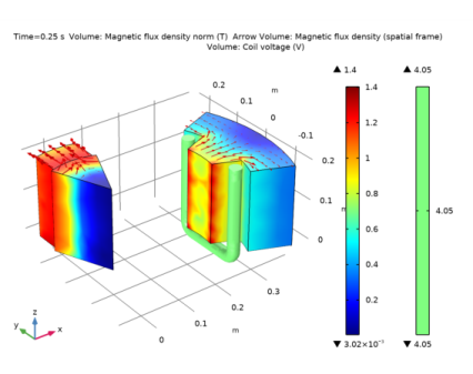
A sector plot of magnetic flux density and the coil voltage is presented in Figure 3. The solution is plotted in the spatial frame, in which the rotor moves.
Figure 3: Sector plot of the magnetic flux density. The global coil voltage is represented as a volume plot on the coil itself.
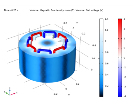
To visualize the solution in the complete geometry, reconstruct it using Sector 3D and Mirror datasets. These specialized datasets create another solution by rotating and mirroring other datasets according to the specification.
To properly account for the antisymmetry, select the Invert phase when rotating check box in the Sector 3D dataset. This functionality changes the sign of the solution when creating adjacent sectors. The resulting plot is shown in Figure 4.
Figure 4: Plot of the magnetic flux density and the global coil voltages in the complete, reconstructed geometry.
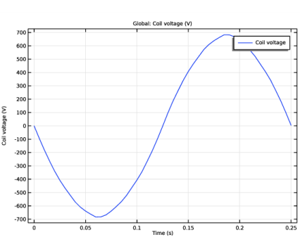
Finally, Figure 5 shows the induced coil voltage as a function of time. The voltage takes into account the number of wires in the multi-turn coil and the symmetry. The simulated voltage is in good agreement with the result from the corresponding 2D model, see Figure 3 in the application Generator in 2D.
Figure 5: Voltage induced in the complete coil as a function of time.
Application Library path: ACDC_Module/Motors_and_Actuators/sector_generator_3d
Modeling Instructions
From the File menu, choose New.
New
In the New window, click  Model Wizard.
Model Wizard
1
In the Model Wizard window, click  3D.
2
In the Select Physics tree, select AC/DC>Electromagnetics and Mechanics>Rotating Machinery, Magnetic (rmm).
3
Click Add.
4
Click  Study.
5
In the Select Study tree, select Preset Studies for Selected Physics Interfaces>Coil Geometry Analysis.
6
Global Definitions
Define Model Parameters: global, constant expressions that can be used anywhere in the application.
Parameters 1
1
In the Model Builder window, under Global Definitions click Parameters 1.
2
In the Settings window for Parameters, locate the Parameters section.
3
Geometry 1
Insert the geometry sequence from a separate file using the Insert Sequence functionality. This functionality copies all the subnodes of the Geometry node in the chosen file to the current model.
1
In the Geometry toolbar, click  Insert Sequence.
2
3
In the Geometry toolbar, click  Build All.
4
Click the  Zoom Extents button in the Graphics toolbar.
The geometry represents a sector of the complete generator, further halved along the xy-symmetry plane. The geometry is composed of two objects, one for the rotor and one for the stator. They have been constructed from the individual components using two Union operations. The geometry is finalized by using Form Assembly, which detects the touching boundaries and creates an Identity Pair connecting them.
Definitions
Proceed to the definition of Selection nodes: named collection of geometric entities (such as domains or boundaries) that can be reused when applying equations, boundary conditions, and other features. New selections can also be obtained by applying more advanced operations on other Selections, such as taking the complement or the adjacent entities. Using Selections simplifies the workflow, especially in models with complex geometries. Explicit selections are named selections in which the entities (domains, in this case) are selected explicitly.
Cylindrical System 2 (sys2)
In the Definitions toolbar, click  Coordinate Systems and choose Cylindrical System.
Explicit 1
In the Definitions toolbar, click  Explicit.
Cylindrical System 2 (sys2)
The cylindrical coordinate system you just added will be used to define the field of the permanent magnets.
Stator Coil
1
In the Model Builder window, under Component 1 (comp1)>Definitions>Selections click Explicit 1.
2
In the Settings window for Explicit, type Stator Coil in the Label text field.
3
Click the  Wireframe Rendering button in the Graphics toolbar.
4
Permanent Magnet
1
In the Definitions toolbar, click  Explicit.
2
In the Settings window for Explicit, type Permanent Magnet in the Label text field.
3
Rotating Domains
1
In the Definitions toolbar, click  Explicit.
2
In the Settings window for Explicit, type Rotating Domains in the Label text field.
3
Definitions
Create a selection for the stationary domains by taking the complement of the rotor selection.
Stationary Domains
1
In the Definitions toolbar, click  Complement.
2
In the Settings window for Complement, type Stationary Domains in the Label text field.
3
Locate the Input Entities section. Under Selections to invert, click  Add.
4
In the Add dialog box, select Rotating Domains in the Selections to invert list.
5
Periodic Condition: Rotor
1
In the Definitions toolbar, click  Explicit.
2
In the Settings window for Explicit, type Periodic Condition: Rotor in the Label text field.
3
Locate the Input Entities section. From the Geometric entity level list, choose Boundary.
4
Periodic Condition: Stator, Scalar Potential
1
In the Definitions toolbar, click  Explicit.
2
In the Settings window for Explicit, type Periodic Condition: Stator, Scalar Potential in the Label text field.
3
Locate the Input Entities section. From the Geometric entity level list, choose Boundary.
4
Periodic Condition: Stator, Vector Potential
1
In the Definitions toolbar, click  Explicit.
2
In the Settings window for Explicit, type Periodic Condition: Stator, Vector Potential in the Label text field.
3
Locate the Input Entities section. From the Geometric entity level list, choose Boundary.
4
Destination
1
In the Definitions toolbar, click  Explicit.
2
In the Settings window for Explicit, type Destination in the Label text field.
3
Locate the Input Entities section. From the Geometric entity level list, choose Boundary.
4
Source
1
In the Definitions toolbar, click  Explicit.
2
In the Settings window for Explicit, type Source in the Label text field.
3
Locate the Input Entities section. From the Geometric entity level list, choose Boundary.
4
Identity Boundary Pair 1 (ap1)
Finally, ensure that the Destination side of the identity pair is on the moving domain. This gives a better performance during the solution.
Check the Source Boundaries and the Destination Boundaries and make sure that the moving domains are in the destination side. The boundaries are numbered progressively with increasing x-coordinate, so the boundaries on the rotor side have lower numbers. Click the Swap Source and Destination button to swap the boundary assignment and put the boundaries with the lower numbers in the destination side.
Add Material
Proceed with the definition of the materials.
1
In the Home toolbar, click  Add Material to open the Add Material window.
2
Go to the Add Material window.
3
4
Click  Add to Component 1 (comp1).
5
In the tree, select AC/DC>Soft Iron (Without Losses).
6
Click  Add to Component 1 (comp1).
7
In the tree, select AC/DC>Hard Magnetic Materials>Sintered NdFeB Grades (Chinese Standard)>N50 (Sintered NdFeB).
8
Click Add to Component in the window toolbar.
9
In the Home toolbar, click  Add Material to close the Add Material window.
Materials
Soft Iron (Without Losses) (mat2)
1
In the Model Builder window, under Component 1 (comp1)>Materials click Soft Iron (Without Losses) (mat2).
2
N50 (Sintered NdFeB) (mat3)
1
In the Model Builder window, click N50 (Sintered NdFeB) (mat3).
2
In the Settings window for Material, locate the Geometric Entity Selection section.
3
From the Selection list, choose Permanent Magnet.
Rotating Machinery, Magnetic (rmm)
Move on to the setup of the physics interface.
Magnetic Flux Conservation: Air Gap
1
In the Model Builder window, under Component 1 (comp1) right-click Rotating Machinery, Magnetic (rmm) and choose Magnetic Flux Conservation.
2
In the Settings window for Magnetic Flux Conservation, type Magnetic Flux Conservation: Air Gap in the Label text field.
3
Magnetic Flux Conservation: Rotor Iron
1
In the Physics toolbar, click  Domains and choose Magnetic Flux Conservation.
2
In the Settings window for Magnetic Flux Conservation, type Magnetic Flux Conservation: Rotor Iron in the Label text field.
3
4
Locate the Constitutive Relation B-H section. From the Magnetization model list, choose B-H curve.
Loss Calculation 1
1
In the Physics toolbar, click  Attributes and choose Loss Calculation.
Set loss model to Bertotti.
2
In the Settings window for Loss Calculation, locate the Loss Model section.
3
From the Loss model list, choose Bertotti.
Ampère’s Law: Stator Iron
1
In the Physics toolbar, click  Domains and choose Ampère’s Law.
2
In the Settings window for Ampère’s Law, type Ampère's Law: Stator Iron in the Label text field.
3
4
Locate the Constitutive Relation B-H section. From the Magnetization model list, choose B-H curve.
Loss Calculation 1
1
In the Physics toolbar, click  Attributes and choose Loss Calculation.
2
In the Settings window for Loss Calculation, locate the Loss Model section.
3
From the Loss model list, choose Bertotti.
Magnet
1
In the Physics toolbar, click  Domains and choose Ampère’s Law.
2
In the Settings window for Ampère’s Law, type Magnet in the Label text field.
3
4
Locate the Coordinate System Selection section. From the Coordinate system list, choose Cylindrical System 2 (sys2).
5
Locate the Constitutive Relation B-H section. From the Magnetization model list, choose Remanent flux density.
Loss Calculation 1
In the Physics toolbar, click  Attributes and choose Loss Calculation.
Coil 1
1
In the Physics toolbar, click  Domains and choose Coil.
2
3
In the Settings window for Coil, locate the Domain Selection section.
4
From the Selection list, choose Stator Coil.
5
Locate the Coil section. From the Conductor model list, choose Homogenized multiturn.
6
From the Coil type list, choose Numeric.
This setting requires to solve a Coil Geometry Analysis preprocessing step.
7
In the Icoil text field, type 0[A].
8
Locate the Homogenized Multiturn Conductor section. In the N text field, type N.
9
In the acoil text field, type d_wire.
Geometry Analysis 1
1
In the Model Builder window, click Geometry Analysis 1.
2
In the Settings window for Geometry Analysis, locate the Coil Geometry section.
3
Find the Symmetry specification subsection. In the FL text field, type 16.
Input 1
1
In the Model Builder window, expand the Geometry Analysis 1 node, then click Input 1.
2
Geometry Analysis 1
The coil domain is only 1/16 of the total length of the coil (due to symmetry). Use the functionality in the Geometry Analysis subfeature to apply the appropriate corrections to the lumped quantities, such as the induced voltage.
In the Model Builder window, click Geometry Analysis 1.
Output 1
1
In the Physics toolbar, click  Attributes and choose Output.
2
Gauge Fixing for A-field 1
The default solver for the 3D Rotating Machinery, Magnetic interface is the direct solver, which gives better performance in time-dependent studies and with the mixed formulation. A direct solver requires that the solution is unique, so it is necessary to apply the Gauge Fixing feature. The Stationary form of Gauge Fixing is enforced so to be able to support regions with zero conductivity.
1
In the Physics toolbar, click  Domains and choose Gauge Fixing for A-field.
2
Click the  Show More Options button in the Model Builder toolbar.
3
In the Show More Options dialog box, in the tree, select the check box for the node Physics>Advanced Physics Options.
4
Sector Symmetry 1
The Sector Symmetry feature sets up the appropriate rotational-periodic coupling at the identity pair.
1
In the Physics toolbar, click  Pairs and choose Sector Symmetry.
2
In the Settings window for Sector Symmetry, locate the Pair Selection section.
3
Under Pairs, click  Add.
4
In the Add dialog box, select Identity Boundary Pair 1 (ap1) in the Pairs list.
5
6
In the Settings window for Sector Symmetry, locate the Sector Settings section.
7
In the nsect text field, type 8.
8
From the Type of periodicity list, choose Antiperiodicity.
9
Click to expand the Constraint Settings section. Select the Use weak constraints check box.
Periodic Condition 1
Apply periodic conditions on the periodic boundaries.
1
In the Physics toolbar, click  Boundaries and choose Periodic Condition.
2
In the Settings window for Periodic Condition, locate the Boundary Selection section.
3
From the Selection list, choose Periodic Condition: Rotor.
4
Locate the Periodic Condition section. From the Type of periodicity list, choose Antiperiodicity.
Periodic Condition 2
1
In the Physics toolbar, click  Boundaries and choose Periodic Condition.
2
In the Settings window for Periodic Condition, locate the Boundary Selection section.
3
From the Selection list, choose Periodic Condition: Stator, Scalar Potential.
4
Locate the Periodic Condition section. From the Type of periodicity list, choose Antiperiodicity.
Periodic Condition 3
1
In the Physics toolbar, click  Boundaries and choose Periodic Condition.
2
In the Settings window for Periodic Condition, locate the Boundary Selection section.
3
From the Selection list, choose Periodic Condition: Stator, Vector Potential.
4
Locate the Periodic Condition section. From the Type of periodicity list, choose Antiperiodicity.
Definitions
Rotating Domain 1
1
In the Definitions toolbar, click  Moving Mesh and choose Rotating Domain.
2
In the Settings window for Rotating Domain, locate the Domain Selection section.
3
From the Selection list, choose Rotating Domains.
4
Locate the Rotation section. From the Rotation type list, choose Specified rotational velocity.
5
From the Rotational velocity expression list, choose Constant revolutions per time.
6
In the f text field, type rpm.
Rotating Machinery, Magnetic (rmm)
1
In the Model Builder window, under Component 1 (comp1) click Rotating Machinery, Magnetic (rmm).
2
In the Settings window for Rotating Machinery, Magnetic, click to expand the Discretization section.
3
From the Magnetic vector potential list, choose Linear.
4
From the Magnetic scalar potential list, choose Linear.
Set the electrical conductivity of air and soft iron to a finite small value (1[S/m]) to improve the numerical stability.
Materials
Air (mat1)
1
In the Model Builder window, under Component 1 (comp1)>Materials click Air (mat1).
2
In the Settings window for Material, locate the Material Contents section.
3
Soft Iron (Without Losses) (mat2)
1
In the Model Builder window, click Soft Iron (Without Losses) (mat2).
2
In the Settings window for Material, locate the Material Contents section.
3
Mesh 1
Set up the mesh for the problem; physics controlled mesh will automatically generate a mesh that is conformal on the two side of the symmetry. This is a strong requirement for all faces where the fields are desribed by vector potential A.
1
In the Model Builder window, under Component 1 (comp1) right-click Mesh 1 and choose Build All.
2
Click the  Go to Default View button in the Graphics toolbar.
Study 1
Complete the definition of the study. After the Coil Geometry Analysis step added earlier, add a Stationary step (to compute the initial values for the transient step) and the main Time Dependent step.
Stationary
In the Study toolbar, click  Study Steps and choose Stationary>Stationary.
Time Dependent
1
In the Study toolbar, click  Study Steps and choose Time Dependent>Time Dependent.
2
In the Settings window for Time Dependent, locate the Study Settings section.
3
In the Output times text field, type range(0,0.005,0.25).
For time-dependent study with finite conductivity in all domains, it is not necessary to use the gauge fixing. Next, it is disabled to make the model cheaper to solve.
4
Locate the Physics and Variables Selection section. Select the Modify model configuration for study step check box.
5
In the Physics and variables selection tree, select Component 1 (comp1)>Rotating Machinery, Magnetic (rmm), Controls spatial frame>Gauge Fixing for A-field 1.
6
Click  Disable.
Solution 1 (sol1)
1
In the Study toolbar, click  Show Default Solver.
Use a stricter tolerance for the stationary step to compute more accurate initial values. This improves the performance of the time dependent solver. Then operate on the setting of the transient solver so to enforce a tighter convergence at each step.
2
In the Model Builder window, expand the Solution 1 (sol1) node, then click Stationary Solver 2.
3
In the Settings window for Stationary Solver, locate the General section.
4
In the Relative tolerance text field, type 1e-6.
5
In the Model Builder window, click Dependent Variables 3.
6
In the Settings window for Dependent Variables, locate the Scaling section.
7
From the Method list, choose None.
8
In the Model Builder window, expand the Study 1>Solver Configurations>Solution 1 (sol1)>Time-Dependent Solver 1 node, then click Direct.
9
In the Settings window for Direct, locate the General section.
10
From the Solver list, choose PARDISO.
11
In the Model Builder window, click Fully Coupled 1.
12
In the Settings window for Fully Coupled, click to expand the Method and Termination section.
13
From the Jacobian update list, choose On every iteration.
14
In the Maximum number of iterations text field, type 25.
15
In the Study toolbar, click  Compute.
Results
Study 1/Solution 1 (sol1)
After the solution is computed, create a sector plot of the magnetic flux density.
Study 1/Solution 1 (Iron)
1
In the Model Builder window, expand the Results>Datasets node.
2
Right-click Results>Datasets>Study 1/Solution 1 (sol1) and choose Duplicate.
3
In the Settings window for Solution, type Study 1/Solution 1 (Iron) in the Label text field.
Visualize the solution in the Spatial frame (the fixed "laboratory" frame), in which the rotor is moving.
Selection
1
In the Results toolbar, click  Attributes and choose Selection.
2
In the Settings window for Selection, locate the Geometric Entity Selection section.
3
From the Geometric entity level list, choose Domain.
4
Study 1/Solution 1 (Coil)
1
Right-click Study 1/Solution 1 (sol1) and choose Duplicate.
2
In the Settings window for Solution, type Study 1/Solution 1 (Coil) in the Label text field.
Selection
1
In the Results toolbar, click  Attributes and choose Selection.
2
In the Settings window for Selection, locate the Geometric Entity Selection section.
3
From the Geometric entity level list, choose Domain.
4
From the Selection list, choose Stator Coil.
Sector Plot
1
In the Model Builder window, under Results click Magnetic Flux Density Norm (rmm).
2
In the Settings window for 3D Plot Group, type Sector Plot in the Label text field.
3
Locate the Data section. From the Dataset list, choose Study 1/Solution 1 (Iron) (sol1).
Multislice 1
1
In the Model Builder window, expand the Sector Plot node.
2
Right-click Multislice 1 and choose Delete.
Streamline Surface 1
In the Model Builder window, right-click Streamline Surface 1 and choose Delete.
Streamline Surface 2
In the Model Builder window, right-click Streamline Surface 2 and choose Delete.
Streamline Surface 3
In the Model Builder window, right-click Streamline Surface 3 and choose Delete.
Volume 1
In the Model Builder window, right-click Sector Plot and choose Volume.
Arrow Volume 1
1
Right-click Sector Plot and choose Arrow Volume.
2
In the Settings window for Arrow Volume, click Replace Expression in the upper-right corner of the Expression section. From the menu, choose Component 1 (comp1)>Rotating Machinery, Magnetic (Magnetic Fields)>Magnetic>rmm.Bx,...,rmm.Bz - Magnetic flux density (spatial frame).
3
Locate the Arrow Positioning section. Find the x grid points subsection. In the Points text field, type 20.
4
Find the y grid points subsection. In the Points text field, type 20.
5
Find the z grid points subsection. From the Entry method list, choose Coordinates.
6
In the Coordinates text field, type 0.2.
Volume 2
1
Right-click Sector Plot and choose Volume.
2
In the Settings window for Volume, click Replace Expression in the upper-right corner of the Expression section. From the menu, choose Component 1 (comp1)>Rotating Machinery, Magnetic (Magnetic Fields)>Coil parameters>rmm.VCoil_1 - Coil voltage - V.
3
Locate the Data section. From the Dataset list, choose Study 1/Solution 1 (Coil) (sol1).
4
In the Sector Plot toolbar, click  Plot.
5
Click the  Zoom Extents button in the Graphics toolbar.
Sector Plot
Reconstruct the complete geometry using Mirror and Sector 3D datasets.
1
In the Model Builder window, click Sector Plot.
2
In the Settings window for 3D Plot Group, locate the Data section.
3
From the Time (s) list, choose 0.08.
4
In the Sector Plot toolbar, click  Plot.
Sector 3D 1
1
In the Results toolbar, click  More Datasets and choose Sector 3D.
2
In the Settings window for Sector 3D, locate the Data section.
3
From the Dataset list, choose Study 1/Solution 1 (Iron) (sol1).
4
Locate the Symmetry section. In the Number of sectors text field, type 8.
5
Click to expand the Advanced section. Select the Invert phase when rotating check box.
Complete Geometry, Iron
1
In the Results toolbar, click  More Datasets and choose Mirror 3D.
2
In the Settings window for Mirror 3D, type Complete Geometry, Iron in the Label text field.
3
Locate the Data section. From the Dataset list, choose Sector 3D 1.
4
Locate the Plane Data section. From the Plane list, choose xy-planes.
5
In the z-coordinate text field, type 0.2.
Sector 3D 2
1
In the Results toolbar, click  More Datasets and choose Sector 3D.
2
In the Settings window for Sector 3D, locate the Data section.
3
From the Dataset list, choose Study 1/Solution 1 (Coil) (sol1).
4
Locate the Symmetry section. In the Number of sectors text field, type 8.
5
Locate the Advanced section. Select the Invert phase when rotating check box.
Complete Geometry, Coil
1
In the Results toolbar, click  More Datasets and choose Mirror 3D.
2
In the Settings window for Mirror 3D, type Complete Geometry, Coil in the Label text field.
3
Locate the Data section. From the Dataset list, choose Sector 3D 2.
4
Locate the Plane Data section. From the Plane list, choose xy-planes.
5
In the z-coordinate text field, type 0.2.
Complete Geometry
1
In the Results toolbar, click  3D Plot Group.
2
In the Settings window for 3D Plot Group, type Complete Geometry in the Label text field.
Volume 1
1
Right-click Complete Geometry and choose Volume.
2
In the Settings window for Volume, locate the Data section.
3
From the Dataset list, choose Complete Geometry, Iron.
4
From the Solution parameters list, choose From parent.
5
Locate the Coloring and Style section. From the Color table list, choose JupiterAuroraBorealis.
Volume 2
1
In the Model Builder window, right-click Complete Geometry and choose Volume.
2
In the Settings window for Volume, click Replace Expression in the upper-right corner of the Expression section. From the menu, choose Component 1 (comp1)>Rotating Machinery, Magnetic (Magnetic Fields)>Coil parameters>rmm.VCoil_1 - Coil voltage - V.
3
Locate the Data section. From the Dataset list, choose Complete Geometry, Coil.
4
From the Solution parameters list, choose From parent.
5
Locate the Coloring and Style section. From the Color table list, choose WaveLight.
Complete Geometry
1
In the Model Builder window, click Complete Geometry.
2
In the Complete Geometry toolbar, click  Plot.
3
Click the  Zoom Extents button in the Graphics toolbar.
Induced Coil Voltage
1
In the Home toolbar, click  Add Plot Group and choose 1D Plot Group.
2
In the Settings window for 1D Plot Group, type Induced Coil Voltage in the Label text field.
Global 1
1
Right-click Induced Coil Voltage and choose Global.
2
In the Settings window for Global, click Replace Expression in the upper-right corner of the y-Axis Data section. From the menu, choose Component 1 (comp1)>Rotating Machinery, Magnetic (Magnetic Fields)>Coil parameters>rmm.VCoil_1 - Coil voltage - V.
3
In the Induced Coil Voltage toolbar, click  Plot.
Next, add the Time to Frequency Losses study to compute the loss.
Add Study
1
In the Home toolbar, click  Add Study to open the Add Study window.
2
Go to the Add Study window.
3
Find the Studies subsection. In the Select Study tree, select Preset Studies for Selected Physics Interfaces>Time to Frequency Losses.
4
Click Add Study in the window toolbar.
5
In the Home toolbar, click  Add Study to close the Add Study window.
Study 2
Step 1: Time to Frequency Losses
1
In the Settings window for Time to Frequency Losses, locate the Study Settings section.
2
From the Input study list, choose Study 1, Time Dependent.
3
In the Electrical period text field, type 0.25.
4
In the Home toolbar, click  Compute.
Results
Volume Integration 1
1
In the Results toolbar, click  More Derived Values and choose Integration>Volume Integration.
2
3
In the Settings window for Volume Integration, locate the Data section.
4
From the Dataset list, choose Study 2/Solution 4 (sol4).
5
Locate the Expressions section. In the table, enter the following settings:
6
Click  Evaluate.
The computed loss power is close to the value computed from the 2D model.
Animation 1
Finally, visualize the rotation of the generator by animating the solution.
1
In the Results toolbar, click  Animation and choose Player.
2
In the Settings window for Animation, locate the Scene section.
3
From the Subject list, choose Complete Geometry.
4
Locate the Playing section. From the Repeat list, choose Forever.
5
In the Graphics toolbar, use the Play and Stop buttons to control the animation.