|
|
|

|
1
|
|
2
|
In the Select Physics tree, select AC/DC>Electromagnetics and Mechanics>Rotating Machinery, Magnetic (rmm).
|
|
3
|
Click Add.
|
|
4
|
Click
|
|
5
|
|
6
|
Click
|
|
1
|
|
2
|
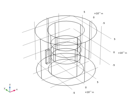
Browse to the model’s Application Libraries folder and double-click the file rotating_machinery_3d_tutorial_geom_sequence.mph.
|
|
3
|
|
4
|
|
5
|
|
1
|
In the Model Builder window, expand the Component 1 (comp1)>Definitions node, then click Identity Boundary Pair 1 (ap1).
|
|
2
|
|
3
|
|
4
|
|
5
|
Click OK.
|
|
6
|
|
7
|
|
8
|
|
9
|
Click OK.
|
|
1
|
|
2
|
|
1
|
|
2
|
|
3
|
In the tree, select Built-in>Air.
|
|
4
|
|
5
|
In the tree, select AC/DC>Copper.
|
|
6
|
|
7
|
In the tree, select AC/DC>Hard Magnetic Materials>Sintered NdFeB Grades (Chinese Standard)>N35 (Sintered NdFeB).
|
|
8
|
|
9
|
|
2
|
|
3
|
|
4
|
|
5
|
Click OK.
|
|
1
|
|
1
|
In the Model Builder window, under Component 1 (comp1) right-click Rotating Machinery, Magnetic (rmm) and choose Magnetic Flux Conservation.
|
|
2
|
In the Settings window for Magnetic Flux Conservation, type Air, formulation for nonconducting domain in the Label text field.
|
|
1
|
|
2
|
In the Settings window for Magnetic Flux Conservation, type Permanent magnet, formulation for nonconducting domain in the Label text field.
|
|
4
|
Locate the Constitutive Relation B-H section. From the Magnetization model list, choose Remanent flux density.
|
|
1
|
|
2
|
|
3
|
|
4
|
|
5
|
In the Show More Options dialog box, in the tree, select the check box for the node Physics>Advanced Physics Options.
|
|
6
|
Click OK.
|
|
7
|
|
8
|
|
1
|
|
3
|
|
4
|
|
5
|
|
1
|
|
2
|
|
3
|
|
4
|
|
5
|
Click OK.
|
|
1
|
|
1
|
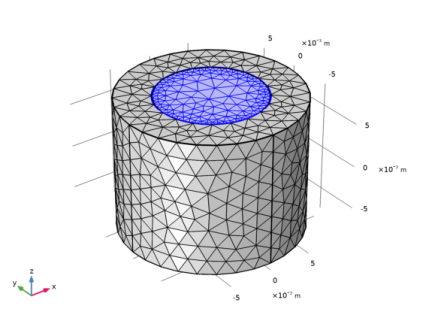
In the Model Builder window, under Component 1 (comp1) right-click Mesh 1 and choose More Operations>Free Triangular.
|
|
2
|
|
3
|
|
1
|
|
2
|
|
3
|
Click the Custom button.
|
|
4
|
|
1
|
|
2
|
|
3
|
|
1
|
|
2
|
|
3
|
Click the Custom button.
|
|
4
|
|
1
|
|
2
|
|
3
|
|
5
|
|
6
|
|
1
|
|
2
|
|
3
|
|
1
|
|
2
|
|
3
|
|
4
|
|
1
|
In the Model Builder window, expand the Boundary Layers 1 node, then click Boundary Layer Properties 1.
|
|
3
|
|
4
|
|
5
|
|
6
|
|
7
|
|
8
|
|
1
|
|
2
|
|
1
|
|
2
|
|
1
|
|
2
|
|
3
|
|
1
|
|
2
|
In the Settings window for Rotating Machinery, Magnetic, click to expand the Discretization section.
|
|
3
|
|
4
|
|
1
|
In the Model Builder window, under Component 1 (comp1)>Rotating Machinery, Magnetic (rmm) click Continuity 1.
|
|
2
|
|
3
|
|
1
|
|
2
|
|
3
|
|
4
|
|
5
|
In the Model Builder window, under Solid copper disk>Solver Configurations>Solution 1 (sol1) click Time-Dependent Solver 1.
|
|
6
|
|
7
|
|
8
|
|
9
|
Find the Algebraic variable settings subsection. From the Error estimation list, choose Exclude algebraic.
|
|
10
|
Click to expand the Output section. Locate the General section. From the Times to store list, choose Steps taken by solver.
|
|
11
|
In the Model Builder window, expand the Solid copper disk>Solver Configurations>Solution 1 (sol1)>Time-Dependent Solver 1 node, then click Fully Coupled 1.
|
|
12
|
|
13
|
|
14
|
In the Model Builder window, under Solid copper disk>Solver Configurations>Solution 1 (sol1)>Time-Dependent Solver 1 click Direct.
|
|
15
|
|
16
|
|
17
|
|
1
|
|
2
|
|
3
|
|
4
|
|
5
|
|
1
|
|
2
|
|
3
|
|
1
|
In the Model Builder window, right-click Currents and solid domain boundaries representation and choose Surface.
|
|
2
|
|
3
|
|
4
|
|
5
|
|
1
|
|
1
|
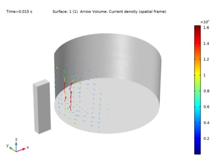
In the Model Builder window, right-click Currents and solid domain boundaries representation and choose Arrow Volume.
|
|
2
|
In the Settings window for Arrow Volume, click Replace Expression in the upper-right corner of the Expression section. From the menu, choose Component 1 (comp1)>Rotating Machinery, Magnetic (Magnetic Fields)>Currents and charge>rmm.Jx,...,rmm.Jz - Current density (spatial frame).
|
|
3
|
Locate the Arrow Positioning section. Find the x grid points subsection. In the Points text field, type 10.
|
|
4
|
|
5
|
|
6
|
|
7
|
|
1
|
|
2
|
|
3
|
|
1
|
|
2
|
|
3
|
|
4
|
|
5
|
|
1
|
|
2
|
|
3
|
|
4
|
Locate the Expressions section. In the table, enter the following settings:
|
|
5
|
|
1
|
Go to the Table window.
|
|
2
|
|
1
|
|
2
|
|
1
|
|
2
|
|
3
|
|
4
|
|
1
|
|
2
|
|
3
|
|
1
|
In the Model Builder window, under Component 1 (comp1)>Electric Currents (ec) click Current Conservation 1.
|
|
2
|
|
3
|
|
1
|
|
2
|
|
3
|
|
4
|
|
1
|
|
1
|
|
1
|
|
2
|
|
3
|
|
4
|
|
1
|
|
2
|
|
3
|
|
4
|
|
1
|
|
2
|
|
3
|
|
1
|
|
2
|
|
3
|
|
4
|
In the Physics and variables selection tree, select Component 1 (comp1)>Rotating Machinery, Magnetic (rmm), Controls spatial frame>External Current Density 1.
|
|
5
|
Click
|
|
6
|
|
7
|
|
1
|
|
2
|
|
3
|
|
4
|
In the Physics and variables selection tree, select Component 1 (comp1)>Rotating Machinery, Magnetic (rmm), Controls spatial frame>External Current Density 1.
|
|
5
|
Click
|
|
6
|
|
7
|
|
1
|
|
2
|
|
3
|
In the Model Builder window, expand the Laminated copper disk>Solver Configurations>Solution 3 (sol3)>Time-Dependent Solver 1 node, then click Laminated copper disk>Solver Configurations>Solution 3 (sol3)>Dependent Variables 2.
|
|
4
|
|
5
|
|
6
|
In the Model Builder window, under Laminated copper disk>Solver Configurations>Solution 3 (sol3) click Time-Dependent Solver 1.
|
|
7
|
|
8
|
|
9
|
Find the Algebraic variable settings subsection. From the Error estimation list, choose Exclude algebraic.
|
|
10
|
|
11
|
|
12
|
Right-click Laminated copper disk>Solver Configurations>Solution 3 (sol3)>Time-Dependent Solver 1 and choose Fully Coupled.
|
|
13
|
|
14
|
|
15
|
In the Model Builder window, under Laminated copper disk>Solver Configurations>Solution 3 (sol3)>Time-Dependent Solver 1 click Direct.
|
|
16
|
|
17
|
|
18
|
|
19
|
|
20
|
|
1
|
|
2
|
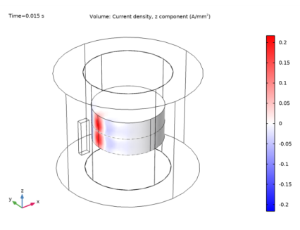
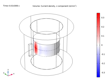
In the Settings window for 3D Plot Group, type Current perpendicular to the insulating plane in the Label text field.
|
|
3
|
|
1
|
|
2
|
|
3
|
|
4
|
|
5
|
|
6
|
|
7
|
|
8
|
Click
|
|
1
|
|
2
|
|
3
|
|
4
|
|
1
|
In the Model Builder window, under Results>Derived Values right-click Volume Integration 1 and choose Duplicate.
|
|
2
|
|
3
|
|
4
|
|
1
|
|
2
|
|
3
|
|
4
|
|
1
|
|
2
|
|
3
|
|
4
|
|
5
|
|
6
|
|
7
|