|
|
|
|
1
|
|
2
|
In the Select Physics tree, select AC/DC>Electromagnetics and Mechanics>Rotating Machinery, Magnetic (rmm).
|
|
3
|
Click Add.
|
|
4
|
Click
|
|
5
|
|
6
|
Click
|
|
1
|
|
2
|
|
1
|
|
2
|
|
3
|
Click Browse.
|
|
4
|
Browse to the model’s Application Libraries folder and double-click the file generator_2d.mphbin.
|
|
5
|
Click Import.
|
|
1
|
|
2
|
|
3
|
|
4
|
|
1
|
|
1
|
|
2
|
|
3
|
In the tree, select Built-in>Air.
|
|
4
|
|
5
|
|
6
|
|
7
|
In the tree, select AC/DC>Hard Magnetic Materials>Sintered NdFeB Grades (Chinese Standard)>N50 (Sintered NdFeB).
|
|
8
|
|
9
|
|
1
|
In the Model Builder window, under Component 1 (comp1)>Materials click Soft Iron (Without Losses) (mat2).
|
|
1
|
|
1
|
|
2
|
|
3
|
|
1
|
|
3
|
|
4
|
|
5
|
|
6
|
|
1
|
|
2
|
|
4
|
Locate the Coordinate System Selection section. From the Coordinate system list, choose Cylindrical System 2 (sys2).
|
|
5
|
|
6
|
|
7
|
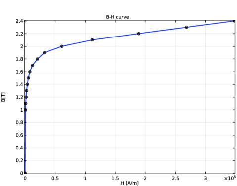
Locate the Constitutive Relation B-H section. From the Magnetization model list, choose Remanent flux density.
|
|
1
|
|
2
|
|
4
|
|
1
|
|
2
|
|
3
|
|
5
|
|
1
|
|
2
|
|
3
|
|
1
|
|
3
|
|
4
|
|
5
|
|
6
|
|
7
|
|
8
|
|
9
|
|
1
|
|
1
|
|
2
|
|
3
|
|
4
|
|
5
|
Click OK.
|
|
1
|
|
2
|
|
3
|
|
1
|
In the Model Builder window, under Component 1 (comp1)>Definitions click Identity Boundary Pair 1 (ap1).
|
|
2
|
|
3
|
|
4
|
|
5
|
Click OK.
|
|
1
|
|
2
|
|
3
|
|
4
|
Click the Custom button.
|
|
5
|
|
1
|
|
2
|
|
3
|
|
4
|
|
5
|
|
6
|
|
1
|
|
2
|
In the Settings window for Rotating Machinery, Magnetic, click to expand the Discretization section.
|
|
3
|
|
4
|
|
5
|
|
6
|
In the Show More Options dialog box, in the tree, select the check box for the node Physics>Advanced Physics Options.
|
|
7
|
Click OK.
|
|
1
|
In the Model Builder window, under Component 1 (comp1)>Rotating Machinery, Magnetic (rmm) click Continuity 1.
|
|
2
|
|
3
|
|
1
|
|
2
|
|
3
|
|
4
|
|
5
|
In the Model Builder window, under Study 1>Solver Configurations>Solution 1 (sol1) click Dependent Variables 2.
|
|
6
|
|
7
|
|
8
|
In the Model Builder window, under Study 1>Solver Configurations>Solution 1 (sol1) click Time-Dependent Solver 1.
|
|
9
|
|
10
|
|
11
|
Find the Algebraic variable settings subsection. From the Error estimation list, choose Exclude algebraic.
|
|
12
|
In the Model Builder window, under Study 1>Solver Configurations>Solution 1 (sol1)>Time-Dependent Solver 1 click Fully Coupled 1.
|
|
13
|
|
14
|
|
15
|
In the Model Builder window, under Study 1>Solver Configurations>Solution 1 (sol1)>Time-Dependent Solver 1 click Direct.
|
|
16
|
|
17
|
|
18
|
|
1
|
In the Model Builder window, expand the Results>Datasets node, then click Magnetic Flux Density Norm (rmm).
|
|
2
|
|
3
|
|
1
|
In the Model Builder window, expand the Magnetic Flux Density Norm (rmm) node, then click Contour 1.
|
|
2
|
|
3
|
|
4
|
|
1
|
|
2
|
|
3
|
|
4
|
|
5
|
|
6
|
In the associated text field, type Time (s).
|
|
7
|
|
8
|
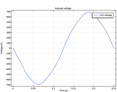
In the associated text field, type Voltage (V).
|
|
1
|
|
2
|
In the Settings window for Global, click Replace Expression in the upper-right corner of the y-Axis Data section. From the menu, choose Component 1 (comp1)>Rotating Machinery, Magnetic (Magnetic Fields)>Coil parameters>rmm.VCoil_3 - Coil voltage - V.
|
|
3
|
|
1
|
|
2
|
|
3
|
Find the Studies subsection. In the Select Study tree, select Preset Studies for Selected Physics Interfaces>Time to Frequency Losses.
|
|
4
|
|
1
|
|
2
|
|
3
|
|
4
|
|
1
|
|
3
|
|
4
|
|
5
|
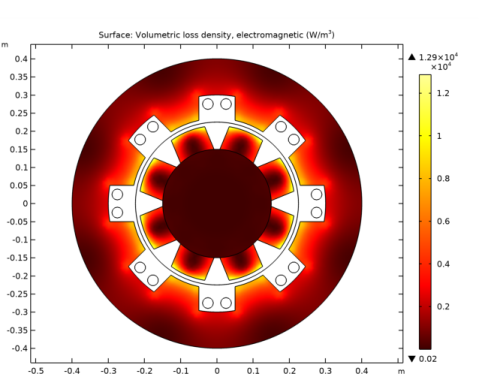
Click Add Expression in the upper-right corner of the Expressions section. From the menu, choose Component 1 (comp1)>Rotating Machinery, Magnetic (Magnetic Fields, No Currents)>Heating and losses>rmm.Qh - Volumetric loss density, electromagnetic - W/m³.
|
|
6
|
Locate the Expressions section. In the table, enter the following settings:
|
|
7
|
Click
|