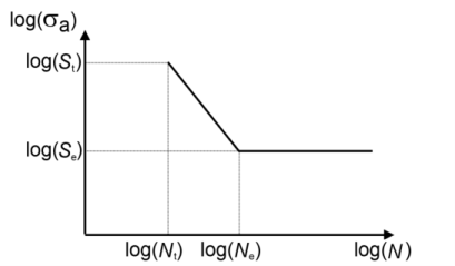
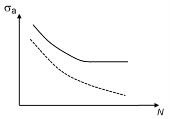
The relation between stress amplitude, σa, and life, N, is one of the oldest methods for fatigue evaluation. It is a very popular method since the relation can be easily obtained from fatigue tests. The relation takes two characteristic shapes, shown in Figure 3-8. The upper shape, which decreases until a point where it becomes a horizontal line, represents materials that have an endurance limit. If the load amplitude in a load cycle is below the endurance limit, the component does not fail in fatigue. If the endurance limit is exceeded, the component does fail in fatigue if the number of load cycles is large enough. The number of cycles where the S-N curve becomes horizontal varies for different materials but is usually in the range of 106 to 108cycles. Several materials do not have an endurance limit and experience fatigue even at low stress amplitudes. This fatigue behavior is demonstrated by the dashed line in Figure 3-8.

where Δσ is the stress range evaluated as the difference between the largest and the smallest stresses experienced during a fatigue cycle.

where σ1 is the largest principal stress, σ3 is the smallest principal stress, σvM is the equivalent stress according to von Mises, and σh is the hydrostatic (or mean) stress.

One of the oldest models for fatigue prediction is the Wöhler curve, also called the S-N curve. It relates the number of cycles, N, to the stress amplitude, σa, when stress cycle is constant. On the equation form it is defined as

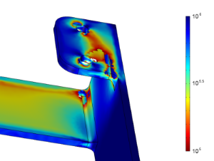
where fSN denotes the S-N function. At low stresses the fatigue life is limited by a Cycle Cutoff. At high stresses, when the stress amplitude exceeds the highest stress as defined by the S-N curve, the fatigue life cannot be determined. No results are computed in such regions. This is demonstrated in Figure 3-9.

Often an S-N curve for the actual operating condition of the component is not available. One way to handle this is to use an S-N curve obtained in the nominal condition and modify it by applying a stress modification factor, k. On the equation form the stress-life relation then becomes

where σf and b are material constants and σa is the stress amplitude. Nf is the number of load cycles to failure, and 2Nf is the number of load reversals. This relation becomes a linear in a log-log diagram and is often utilized in engineering applications. At low stresses the fatigue life is limited by a Cycle Cutoff.

In cases where accurate stress-life data is missing, an approximate method can be applied. Since the Basquin equation is a linear relation in the log-log space and the endurance limit is a straight line, a bilinear approximate of an S-N curve can be constructed. This requires knowledge of the endurance limit and the transition between the high-cycle fatigue (HCF) and the low-cycle fatigue. In a fatigue life (N) versus stress amplitude (σa) graph, the bilinear relation can be constructed as shown Figure 3-10.

The transition stress between LCF and HCF is denoted by St, the transition life is denoted by Nt, and the endurance limit or the endurance stress is denoted by Se. The point that defines a knee on the S-N curve is denoted Ne and is called the endurance life. Often the key parameters of the approximate curve are expressed using the ultimate tensile stress, Su. In steel, for example, the values are roughly St = 0.9 ⋅ Su, Nt = 103 cycles, and Se = 0.5 ⋅ Su, Ne = 106 cycles.

The amplitude stress that is being used in fatigue evaluation using the S-N Curve model, the Basquin model, or the Approximate S-N Curve model can be modified to account for the mean stress. The mean stress σm is defined as the average of the minimum and maximum stresses during a load cycle. The scalar stress measure used is the same as in for defining the amplitude stress.

If you select Gerber as Method, the amplitude stress is modified using the mean stress as

where σu is an ultimate tensile strength that you need to specify.

If you select Goodman as Method, the amplitude stress is modified using the mean stress as

If you select Soderberg as Method, the amplitude stress is modified using the mean stress as

where σys is a yield stress that you need to specify. The Soderberg method is similar to the Goodman method in the sense that the interaction curve is a straight line. The Soderberg method is however more conservative, since it predicts that failure when the mean stress is at the yield limit, rather than the at the ultimate tensile stress.