Many materials have a distinct elastic regime, in which the deformations are recoverable and path independent. When the stresses exceed a certain level, the yield limit, permanent plastic strains will appear.

The elastic part of the constitutive relation can be described by either a Linear Elastic Material, Nonlinear Elastic Materials, or by Hyperelastic Material Models.

where fc can be a constant value (for perfectly plastic materials), or a variable for strain-hardening materials. The yield surface F is a surface in the space of principal stresses, in which the elastic regime (F ≤ 0) is enclosed.

For brittle materials, the yield surface represents a failure surface, which is a stress level at which the material collapses instead of deforms plastically.

For isotropic plasticity, the plastic potential Qp is written in terms of at most three invariants of Cauchy’s stress tensor

The trace of the incremental plastic strain tensor, which is called the volumetric plastic strain rate , is only a result of dependence of the plastic potential on the first invariant I1(σ), since ∂J2/∂σ and ∂J3/∂σ are deviatoric tensors

A common measure of inelastic deformation is the effective plastic strain rate, which is defined from the plastic shear components

For metal plasticity under the von Mises or Tresca criteria, the volumetric plastic strain rate is always zero because the plastic potential is independent of the invariant I1(σ). This is known as J2 plasticity.

Incompressible plastic deformation is experimentally observed in metals, but this is not the case for most materials used in geotechnical applications. For instance, a nonzero volumetric plastic strain is explicitly used in Porous Plasticity and Elastoplastic Soil Models.

where σys is the yield stress. The scalar function is called equivalent stress. The default form of the equivalent stress is the von Mises stress, which is often used in metal plasticity:

Other expressions can be defined, such as Tresca stress, Hill orthotropic plasticity, or a user defined expression.

the effective (von Mises) stress σmises, or other invariants, principal stresses, or stress tensor components.

The von Mises criterion suggests that the yielding of the material begins when the second deviatoric stress invariant J2 reaches a critical value. This criterion can be written in terms of the elements of Cauchy’s stress tensor (Ref. 1)

where σys is the yield stress level (yield stress in uniaxial tension).

The Tresca criterion is a hexagonal prism with its axis equally inclined to the three principal stress axes. When the principal stresses fulfill σ1 ≥ σ2 ≥ σ3, this criterion is written as

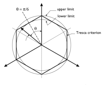
By using the representation of principal stresses in term of the invariants J2 and the Lode angle 0 ≤ θ ≤ π/3, this criterion can alternatively be written as

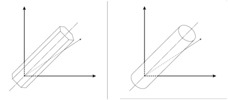
The maximum shear stress is reached at the meridians (θ = 0 or θ = π/3). The Tresca criterion can be circumscribed by setting the Lode angle θ = 0, or equivalently, by a von Mises criterion

The minimum shear is reached at θ = π/6, so the Tresca criterion can be inscribed by setting a von Mises criterion

When dealing with soils, the parameter k is also called undrained shear strength.

The von Mises and Tresca criteria are independent of the first stress invariant I1 and are mainly used for the analysis of plastic deformation in metals and ductile materials, though some researchers also use these criteria for describing fully saturated cohesive soils under undrained conditions. The von Mises and Tresca criteria belong to what researchers call volume preserving or J2 plasticity, as the plastic flow is independent on the mean pressure.

The modeling of plastic deformation in soils, porous metals and aggregates has a main difference with respect to traditional metal plasticity; the yield function and plastic potential are not only defined in terms of the deviatoric stress tensor (or the deviatoric stress invariant J2), but also include dependencies on the hydrostatic pressure.

A key concept for porous plasticity models is the evolution of the relative density, which is the solid volume fraction in a porous mixture. The relative density is related to the porosity (or void volume fraction) by

Shima and Oyane (Ref. 8) proposed a yield surface for modeling the compaction of porous metallic structures fabricated by sintering. The criterion can be applied for powder compaction at both low and high temperatures. The yield function and associated plastic potential is defined by an ellipsoid in the stress space. The plastic potential Qp is written in terms of both von Mises equivalent stress and mean pressure, and it also considers isotropic hardening due to changes in porosity. The plastic potential is defined by

here, σe is the equivalent stress, σ0 is the yield stress, pm is the pressure, and ρrel is the relative density. The material parameters α, γ, and m are obtained from curve fitting experimental data. Typical material parameter values for copper aggregates are α = 6.2, γ = 1.03, and m = 5.

Gurson criterion (Ref. 9) consists in a pressure dependent yield function to describe the constitutive response of porous metals, this yield function is derived from the analytical expression of an isolated void immersed in a continuum medium. The void volume fraction, or porosity φ, is chosen as main variable. The yield function and associated plastic potential is not an ellipse in the stress space, as in Shima-Oyane Criterion, but it is defined in terms of the hyperbolic cosine function. The plastic potential for Gurson criterion reads

here, σe is the equivalent stress, σ0 is the initial yield stress, pm is the pressure, and is the porosity.

Tvergaard and Needleman modified Gurson Criterion for porous plasticity to include parameters to better fit experimental data (Ref. 10-11). The resulting criterion is called in the literature Gurson-Tvergaard-Needleman (GTN) criterion. The plastic potential for GTN criterion reads

here, σe is the equivalent stress, σ0 is the initial yield stress, pm is the pressure, and is the effective void volume fraction (effective porosity). Typical correction parameter values are q1 = 1.5, q2 = 1.03, and q3 = q12.

The effective void value fraction (or effective porosity) used in the plastic potential is a function of the current porosity and other material parameters:

Since typical values for the parameters are q3 = q12, the maximum porosity value is given by .

The Fleck-Kuhn-McMeeking criterion (Ref. 13), also called FKM criterion, was developed to model the plastic yielding of metal aggregates of high porosity. The yield function and associated plastic potential is derived from expressions for randomly distributed particles. The criterion is considered relevant for aggregates with porosity between 10% and 35%. The plastic potential for FKM criterion reads

here, σe is the equivalent stress and pm is the pressure. The flow strength of the material under hydrostatic loading, pf, is computed from

here, σ0 is the initial yield stress, and is the void volume fraction (porosity). The maximum void volume fraction typically takes the value of 36%, the limit of dense random packing of sintered powder.

The FKM-GTN criterion is a combination of the Fleck-Kuhn-McMeeking Criterion and Gurson-Tvergaard-Needleman Criterion, intended to cover a wider range of porosities (Ref. 14-15). The GTN model is used for low void volume fractions (porosity lower than 10%), and for void volume fractions higher than 25%, the FKM criterion is used. In the transition zone, a linear combination of both criteria is used.

Since the relative density is related to the porosity by ρrel = 1 − , the change in porosity is also controlled by the change in plastic volumetric strain

here, εN is the mean strain for nucleation, fN is the void volume fraction for nucleating particles, and sN is the standard deviation. Typical values for these parameters are εN = 0.04, sN = 0.1, and fN = 0.04. It is assumed that nucleation appears only in tension, and that there is no nucleation in compression.

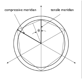
here, kw is a material parameter, is the current porosity, nD is a deviatoric tensor coaxial to the stress tensor, and is the plastic strain rate, which depends on the porous plasticity model. The weight w is computed from stress invariants as

where θ is the Lode angle. The weight variable has a value of w = 0 at the compressive and tensile meridians (θ = 0 and θ = π/3), and it attains its maximum w = 1 for θ = π/6.

here, τ is the shear stress, c the cohesion, and denotes the angle of internal friction.

The Mohr-Coulomb criterion can be written in terms of the invariants I1 and J2 and the Lode angle 0 ≤ θ ≤ π/3 (Ref. 1, Ref. 9) when the principal stresses are sorted as σ1 ≥ σ2 ≥ σ3. The yield function then reads

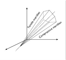
The tensile meridian is defined when θ = 0 and the compressive meridian when θ = π/3.

In the special case of frictionless material, (, α = 0, k = c), the Mohr-Coulomb criterion reduces to a Tresca’s maximum shear stress criterion, (σ1 − σ3) = 2k or equivalently

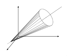
The Mohr-Coulomb criterion causes numerical difficulties when treating the plastic flow at the corners of the yield surface. The Drucker-Prager model neglects the influence of the invariant J3 (introduced by the Lode angle) on the cross-sectional shape of the yield surface. It can be considered as the first attempt to approximate the Mohr-Coulomb criterion by a smooth function based on the invariants I1 and J2 together with two material constants (which can be related to Mohr-Coulomb’s coefficients)

This is sometimes also called the extended von Mises criterion, since it is equivalent to the von Mises criterion for metals when setting α = 0.

The matching at the tensile meridian (θ = 0) comes from setting

in the Mohr-Coulomb criterion, and the matching at the compressive meridian (θ = π/3) from setting

In the special case of frictionless material, (, α = 0, ), the Drucker-Prager criterion reduces to the von Mises criterion

The Mohr-Coulomb yield criterion is sometimes used with a nonassociated plastic potential. This plastic potential could be either a Drucker-Prager criterion, or the same Mohr-Coulomb yield function but with a different slope with respect to the hydrostatic axis, in which case the angle of internal friction is replaced by the dilatation angle, which is normally smaller (Ref. 5).

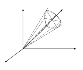
The elliptic cap is an elliptic yield surface of semi-axes as shown in Figure 3-10. The initial pressure pa (SI units: Pa) denotes the pressure at which the elastic range circumscribed by either a Mohr-Coulomb pyramid or a Drucker-Prager cone is not valid any longer, so a cap surface is added. The limit pressure pb gives the curvature of the ellipse, and denotes the maximum admissible hydrostatic pressure for which the material starts deforming plastically. Pressures higher than pb are not allowed.

Note that the sign convention for the pressure is taken from the Structural Mechanics Module: positive sign under compression, so pa and pb are positive parameters. Figure 3-10 shows the cap in terms of the variables p and q

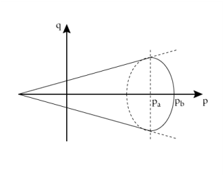
the point (pa, qa) in the Haigh–Westergaard coordinate system is where the elliptic cap intersects either the Mohr-Coulomb or the Drucker-Prager cone.

here, pb0 is the initial value for the limit pressure pb, Kiso is the isotropic hardening modulus, εpvol the volumetric plastic strain, and εpvol,max the maximum volumetric plastic strain. Instead of providing the value for the initial pressure pa (SI units: Pa), the ellipse’s aspect ratio R is entered.

Note that the volumetric plastic strain εpvol is negative in compression, so the limit pressure pb is increased from pb0 as hardening evolves.

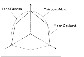
Matsuoka and Nakai (Ref. 3) discovered that the sliding of soil particles occurs in the plane in which the ratio of shear stress to normal stress has its maximum value, which they called the mobilized plane. They defined the yield surface as

where the parameter μ = (τ/σn)STP equals the maximum ratio between shear stress and normal stress in the spatially mobilized plane (STP-plane), and the invariants are applied over the effective stress tensor (this is the Cauchy stress tensor minus the fluid pore pressure).

where I1 and I3 are the first and third stress invariants, respectively, and k is a parameter related to the direction of the plastic strain increment in the triaxial plane. The parameter k can vary from 27 for hydrostatic stress conditions (σ1 = σ2 = σ3), up to a critical value kc at failure. In terms of the invariants I1, J2,and J3, this criterion can be written as

It appears that the Mohr-Coulomb and Drucker-Prager criteria predict tensile strengths larger than the experimental measurements on soil samples. This discordance can be mended by the introduction of a tension cut-off criterion.

The Rankine criterion states that a material stops deforming elastically when the largest principal stress σ1 reaches a maximum tensile stress, also called tension cut-off limit σt.

For soils and clays, the maximum tensile stress can be estimated from the material parameters, such as the cohesion c and the friction angle φ. For instance, the tip of the cone in Mohr-Coulomb criterion is reached when

The Mohr-Coulomb criterion together with a tension cut-off is sometimes called modified Mohr-Coulomb criterion (Ref. 19).

here, σm is the maximum mean stress and p = -I1/3 is the pressure, which is negative in tension.

Hill (Ref. 6, Ref. 7) proposed a quadratic yield function (and associated plastic potential) in a local coordinate system given by the principal axes of orthotropy ai

The six parameters F, G, H, L, M, and N are related to the state of anisotropy. As with isotropic plasticity, the elastic region Qp < 0 is bounded by the yield surface Qp = 0.

Hill noticed that the parameters L, M, and N are related to the yield stress in shear with respect to the axes of orthotropy ai, thus they are positive parameters

Here, σysij represents the yield stress in shear on the plane ij.

The material parameters σys1, σys2, and σys3 represent the tensile yield stress in the direction, a1, a2, and a3, and they are related to Hill’s parameters F, G, and H as

Note that at most one of the three coefficients F, G, and H can be negative.

In order to define a yield function and plastic potential suitable for isotropic or kinematic hardening, the average initial yield stress σys0 is calculated from the Hill’s parameters F, G, and H (this is equivalent to the initial yield stress σys0 in von Mises plasticity)

Defining Hill’s equivalent stress as (Ref. 7)

Isotropic hardening is then applied on the average yield stress variable σys0, by using the plastic potential

now depends on the initial yield stress σys0, the hardening function σh, and the effective plastic strain εpe.

In this case the plasticity algorithm solves either the associated or nonassociated flow rule for the plastic potential Qp

In the settings for plasticity you specify the equivalent stress for the yield function from von Mises stress, Tresca stress, Hill equivalent stress, or a user defined expression; and σys0 is the initial yield stress that defines the onset of plastic deformation.

where the yield stress σys(εpe) now depends on the effective plastic strain εpe.

The yield stress σys(εpe) is then a function of the effective plastic strain and the initial yield stress σys0

here, the isotropic hardening modulus Eiso is calculated from

For linear isotropic hardening, the isotropic tangent modulus ETiso is defined as (stress increment / total strain increment). A value for ETiso is entered in the isotropic tangent modulus section for the Plasticity node. The Young’s modulus E is taken from the parent material (Linear Elastic, Nonlinear Elastic or Hyperelastic material model). For orthotropic and anisotropic elastic materials, E represents an effective Young’s modulus.

In the Ludwik model for nonlinear isotropic hardening, the yield stress σys(εpe) is defined by a nonlinear function of the effective plastic strain. The Ludwik equation (also called Ludwik-Hollomon equation) for isotropic hardening is given by the power law

Here, k is the strength coefficient and n is the hardening exponent. Setting n = 1 would result in linear isotropic hardening.

Similar to the Ludwik hardening model, the yield stress σys(εpe) in the Johnson-Cook model is defined as a nonlinear function of the effective plastic strain εpe given by a power law. The difference is that effects of the strain rate are included in the model. The yield stress and hardening function is given by

The Johnson-Cook model also adds the possibility to include thermal softening by including a function which depends on the normalized homologous temperature Th. It is a function of the current temperature T, the melting temperature of the metal Tm, and a reference temperature Tref

As a default, this dependency follows a power law, . The softening function f(Th) should have the properties f(Th<0) = 0 and f(Th>1) = 1.

The strain rate strength coefficient C and the reference strain rate in the Johnson-Cook model are obtained from experimental data. The flow curve properties are normally investigated by conducting uniaxial tension tests in a temperature range around half the melting temperature Tm, and subjected to different strain rates like 0.1/s, 1/s, and 10/s.

It should be noted that the intent of the strain rate dependent term in Equation 3-35 is to capture the hardening at high strain rates. If extrapolated to very low strain rates, a low or even negative yield stress will be predicted. Low strain rates can however be expected in some regions in a general finite element model. To resolve this, the material model as implemented, never evaluates the logarithmic term to a value smaller than zero. This means that the reference strain rate must be considered the quasistatic limit. Below this strain rate, the hardening function will be a strain rate independent, but temperature dependent, Ludwik law:

For nonsaturating materials, the Swift power-law equation relates the initial yield stress σys0 and the isotropic hardening σh, to the effective plastic strain as

here, k is the strength coefficient, n is the hardening exponent, and ε0 is a reference strain. Noting that at zero plastic strain the initial yield stress is related to the strength coefficient and hardening exponent as

The Voce rule for nonlinear isotropic hardening is intended for materials that exhibit a saturating evolution of hardening. The isotropic hardening σh is exponentially related to the effective plastic strain as

The yield stress σys(εpe) is then defined as

The value of the saturation exponent parameter β determines the saturation rate of the hysteresis loop for cyclic loading. The saturation flow stress σsat characterizes the maximum distance by which the yield surface can expand in the stress space. For values εpe >> 1/β, the yield stress saturates to

where σ∝ is the steady-state flow stress, m the saturation coefficient and n the saturation exponent. For values mεpen >> 1 the yield stress saturates to

In this case, define the (usually nonlinear) hardening function σh(εpe) such that the yields stress reads

Here, σys is the yield stress (which may include a linear or nonlinear isotropic hardening model), and the equivalent stress is either the von Mises, Tresca, or Hill stress; or a user defined expression. The stress tensor used in the yield function is shifted by what is usually called the back stress, σback.

The back stress is generally not only a function of the current plastic strain but also of its history. In the case of linear kinematic hardening, the back stress σback is a linear function of the plastic strain tensor εp, this is also known as Prager’s hardening rule.

where the kinematic hardening modulus Ck is calculated from

The value for Ek is entered in the kinematic tangent modulus section and the Young’s modulus E is taken from the linear or nonlinear elastic material model. For orthotropic and anisotropic elastic materials, E represents an averaged Young’s modulus. Note that some authors define the kinematic hardening modulus as Hk = 2/3Ck.

Armstrong and Frederick (Ref. 1) added memory to Prager’s linear kinematic hardening model. This nonlinear kinematic hardening model allows to capture the Bauschinger effect and nonlinear behavior by non symmetrical tension-compression loading.

The nonlinear evolution of the back stress σback is governed by the rate

here, Ck is the kinematic hardening modulus, γk is a kinematic hardening parameter, and εpe the effective plastic strain. Setting γk = 0 recovers Prager’s rule for linear kinematic hardening.

To solve this rate, internal degrees of freedom are added to account for the back stress components. In order to have the same units as used for the plastic strain, the algorithm solves for the back strain εback as proposed in (Ref. 2), which is related to the back stress as

Chaboche (Ref. 2) proposed a nonlinear kinematic hardening model based on the superposition of N back stress tensors

each of these back stress tensors σback,i follows a nonlinear Frederick-Armstrong kinematic hardening rule

Practitioners would normally select γk = 0 for one of the back stress equations, thus recovering Prager’s linear rule for that branch

The back stress tensor σback is then defined by the superposition of N back stress tensors

As done for Armstrong-Frederik kinematic hardening, the algorithm solves for the back strain tensors εback,i instead of the back stress tensors. The change of variables is

There are two implementations of plasticity available in COMSOL Multiphysics. One is based on the additive decomposition of strains, which is the most suitable approach in the case of small strains, and the other one is based on the multiplicative decomposition of the deformation gradient, which is more suitable when large plastic strains occurs. The additive and multiplicative decomposition of strains is described in Inelastic Strain Contributions.

When small plastic strain is selected as the plasticity model, an additive decomposition is used. If the elastic or plastic strains are large, the additive decomposition might produce incorrect results. As an example, the volume preservation, which is an important assumption in metal plasticity, will no longer be respected. The additive decomposition of strains is however widely used both for metal and soil plasticity.

When large plastic strain is selected as the plasticity model, the total deformation gradient tensor is multiplicatively decomposed into an elastic deformation gradient and a plastic deformation gradient.

The flow rule defines the relationship between the increment of the plastic strain tensor  and the current state of stress, σ, for a yielded material subject to further loading. When Small plastic strain is selected as the plasticity model for the Plasticity node, the direction of the plastic strain increment is defined by

Here, λ is a positive multiplier (also called the consistency parameter or plastic multiplier), which depends on the current state of stress and the load history, and Qp is the plastic potential.

The direction of the plastic strain increment is perpendicular to the surface (in the hyperspace spanned by the stress tensor components) defined by the plastic potential Qp.

The plastic multiplier λ is determined by the complementarity or Kuhn-Tucker conditions

where Fy is the yield function. The yield surface encloses the elastic region defined by Fy < 0. Plastic flow occurs when Fy = 0.

If the plastic potential and the yield surface coincide with each other (Qp = Fy), the flow rule is called associated, and the rate in Equation 3-37 is solved together with the conditions in Equation 3-36.

For a nonassociated flow rule, the yield function does not coincide with the plastic potential, and together with the conditions in Equation 3-36, the rate in Equation 3-38 is solved for the plastic potential Qp (often, a smoothed version of Fy).

The evolution of the plastic strain tensor (with either Equation 3-37 or Equation 3-38, plus the conditions in Equation 3-36) is implemented at Gauss points in the plastic element elplastic.

When Large plastic strain is selected as the plasticity model for the Plasticity node, a multiplicative decomposition of deformation (Ref. 3, Ref. 4, and Ref. 5) is used, and the associated plastic flow rule can be written as the Lie derivative of the elastic left Cauchy-Green deformation tensor Bel:

The plastic multiplier λ and the yield function Φ (written in terms of the Kirchhoff stress tensor τ) satisfy the Kuhn-Tucker condition, as done for infinitesimal strain plasticity

The Lie derivative of Bel is then written in terms of the plastic right Cauchy-Green rate

By using Equation 3-39 and Equation 3-40, the either associated or nonassociated plastic flow rule for large strains is written as (Ref. 4)

together with the Kuhn-Tucker conditions for the plastic multiplier λ and the yield function Fy

For the associated flow rule, the plastic potential and the yield surface coincide with each other (Qp = Fy), and for the nonassociated case, the yield function does not coincide with the plastic potential.

In COMSOL Multiphysics, the elastic left Cauchy-Green tensor is written in terms of the deformation gradient and the right Cauchy-Green tensor, so Bel = FCp−1FT. The flow rule then reads

The plastic flow rule is then solved at Gauss points in the plastic element elplastic for the inverse of the plastic deformation gradient Fp−1, so that the variables in Equation 3-43 are replaced by

After integrating the flow rule in Equation 3-43, the plastic Green-Lagrange strain tensor is computed from the plastic deformation tensor

and the elastic Green-Lagrange strain tensor is computed from the elastic deformation gradient tensor Fel = FFp−1

where “old” denotes the previous time step and Λ = λΔt, where Δt is the pseudo-time step length.

For large plastic strains, Equation 3-43 is numerically solved with the so-called exponential mapping technique

For each Gauss point, the plastic state variables (εp or Fp−1, depending on whether small strain or large strain plasticity is selected) and the plastic multiplier, Λ, are computed by solving either of the above time-discretized flow rules together with the complementarity conditions

This is done as follows (Ref. 3):

As plasticity is rate independent, the plastic dissipation density Wp is obtained after integrating an extra variable in the plastic flow rule.

The total energy dissipated by plasticity in a given volume can be calculated by a volume integration of the plastic dissipation density Wp.