Introduction to Solvers and Studies
The process of solving a problem in COMSOL Multiphysics is a hierarchy. The Study node () is the coarsest level (the top level). It contains the least amount of detail and defines a Study branch (see Branches and Subbranches in the Tree Structure).
Figure 20-1: An example of the hierarchy under the Study node. This is the completed study and solver sequence for the Diagonal Mounting Detail of a Communication Mast model from the COMSOL Multiphysics Applications Libraries. Some hierarchical categories for this sequence are shown.
Adding a Study and Study Steps
When creating a new model, you can add any of the predefined Study and Study Step Types. At any time you can also add studies (see The Add Study Window). However you choose to add a study, a study node is added to 
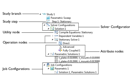
The Model Builder including a corresponding study step (for example, Stationary in Figure 20-1), and in some cases, additional study steps. The study step represents the next level of detail.
Defining Study Steps and Creating Solver Configurations
Most study steps are used to control the form of the equations, what physics interfaces are included in the computation, and what mesh is used. A study step Settings window has a Physics and Variables Selection section where inclusion and exclusion of physics interfaces and variables can be adjusted and set. There are also Common Study Step Settings for many of the study features added to a sequence.
Study steps correspond to part of a solver configuration (solver sequence), which is the next level of detail. There are also study steps for cluster computing, for example, which correspond to part of the Job Configurations.
Solver Configurations contain nodes that define variables to solve for, the solvers and settings, and additional sequence nodes for storing the solution, for example (see Figure 20-1). The solvers also have nodes that can control the solver settings in detail. Knowing The Relationship Between Study Steps and Solver Configurations is useful to help define and edit the settings before computing a solution. Bear in mind, however, that the default solver settings defined by the study usually provide a good starting point.
Computing the Solution
Once the studies are added and defined, the simplest option to compute the solution is to right-click the Study node for a predefined study type and select Compute (). This generates the default solver configuration for the corresponding study steps and computes the solution. There are a variety of techniques you can use while Computing a Solution, including many custom adjustments.
Controlling and Customizing Solver Settings
The settings can also be controlled at any level of detail. For example, you can add individual study steps when there is not a predefined study type that corresponds to the simulations you are interested in doing. Also, by changing the settings in the solver configuration you can, for example, control the desired tolerance for the error in the solution or which time-integration method or linear solver to use.
Solver Operation, Attribute, and Utility Nodes
There are different groups of feature types you can use to customize and fine tune the model. There are three classes of features that are subnodes to a Solution node. See Figure 20-1 for examples:
Operation nodes (typically solvers) produce solutions as output. In particular, the output from the operation node that ran last is available for results analysis and visualization. See Solution Operation Nodes and Solvers.
Attribute nodes hold properties that control the behavior of operation features. See Solution Attribute Nodes.
Utility nodes handle special types of operations. Applicable solution utility nodes are available from the Solver>Other submenu. See Solution Utility Nodes.
Some of the settings in subnodes are synchronized with the corresponding Study setting. They are unavailable by default and can only be controlled from the subnode by changing the Defined by study step setting to User defined.
There are also Study Extension Steps (Parametric Sweep and Optimization) and categories of Advanced Study Extension Steps ( Parametric, Batch, and Cluster Computing) for additional settings customization and extensions of a study.
For some modules, more settings are available with respect to Harmonic Perturbation, Prestressed Analysis, and Small-Signal Analysis.
About Solver Commands and Solution Object Data in the COMSOL Multiphysics Programming Reference Manual.
Multiple Study Steps vs. Multiple Studies
You can create multiple studies with one or more study step in each study. There are some aspects to consider when choosing to use multiple study steps in a single study versus multiple studies, each with a single or just a couple of study steps.
The main advantage of using multiple study steps is that initial conditions are automatically taken from the preceding step. It is also easier to run the whole sequence in one go.
When you use separate studies, you have to use more settings in the main Study node to point to the results in the preceding study. This approach can be useful if you need to examine the results of one study step before proceeding to the next. See Study Reference for information about referencing another study.
There are also some differences in how results are stored and shown. In a sequence with several study steps, you typically only see the results of the last step as a default. You can, however, access the results of the intermediate steps manually.