Computing a Solution
A solution can be computed in a few ways depending on the sequence implemented for a model.
The Difference Between Computing a Study, Solver, or Job
There are conceptual differences between computing, or running, a study versus running a solver configuration or a job configuration. When a solver configuration or job configuration is run, no nodes are added or removed; it is computed “as is.”
Running a study, on the other hand, can be different. When you compute a Study, it always runs the enabled configurations (see below). What the Study runs can be a Job or a Solver (for example, a Stationary Solver) depending on the study configuration. If a Job is run, it typically also means that a solver is also run (by the job). But before the study runs a job or a solver, it reconstructs the (enabled) configurations from scratch. An exception to this rule is when the enabled configurations are edited (an asterisk indicates this; see Figure 20-7 for an example), in which case the sequences are computed “as is.”
About Enabled Study or Solver Sequences
The particular sequence that is Enabled and runs when selecting Compute has a green border around its icon (). You can disable an enabled sequence by right-clicking the node and selecting Disable (which removes the green border). If no sequence is enabled when the study or solver configuration attempts to generate a sequence, a new sequence with default settings is generated. Only one sequence per study can be enabled. For job configurations, the sequence here means a unique path defined from a solver sequence to a job configuration and possibly another job configuration pointing to that job configuration, and so on. Also see Figure 20-6 for other examples of enabled sequences.
Computing a Study or Solver
The most straightforward method to compute a solution is to right-click the Study node () and select Compute () or press F8. You can also click Compute () on the Main and Study toolbars and on the toolbar at the top of the study steps’ and solver nodes’ Settings windows.
By default, a study creates a Solution dataset and plot groups with results plots suitable for the physics interfaces for which you compute the solution. If you do not want to generate plots automatically, clear the Generate default plots check box in the Study Settings section in the main Study node’s Settings window.
If the study contains more than one study step, and you want to compute only a part of the study steps, right-click a study step and select:
Compute Selected Step () (or press F7) to compute just the selected study step.
Compute to Selected () to compute from the first to the selected study step.
Compute from Selected () to compute for all study steps from the selected study step to the last.
If you show the solver sequences under Solver Configurations, you can right-click any node in a solver sequence and select:
Compute () (or press F8) to compute the entire solver sequence.
Compute to Selected () (or press F7) to compute the solver sequence from the top down to the selected node.
Compute from Selected () to compute from the Compile Equations node () that is associated with the selected node down to the end of the solver sequence.
Updating a Solution
To update the solution for a study to use the current values of parameters and user-defined variables, right-click the Study node and select Update Solution () (or press F5).
Updating the solution updates the current study (if selected) or all studies if no study is selected. This is useful in the following situations when you have:
In all these cases, the COMSOL software passes or interpolates the solution to the resulting datasets but does not recompute it to reflect any changes in variables, equations, mesh, or geometry.
Computing a Solver Configuration
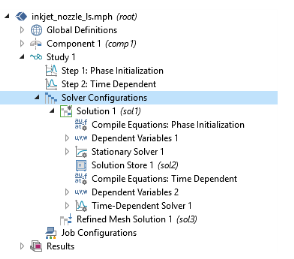
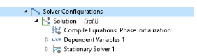
When you have added study steps to a study, a Solver Configurations (and maybe a Job Configurations) sequence is generated when the Study is computed. The Solver Configurations branch represents the solvers, dependent variables and degrees of freedom, and other study-related functionality that the study steps require.
A Solver Configurations or Job Configurations node displays automatically if it has content. Otherwise, if you click the Show More Options button () and select Solver and Job Configurations in the Show More Options dialog box, it is available as an option from the context menu.
In some cases, the default settings in the study steps are not sufficient to specify the details of how to obtain a solution. In this case you can edit the sequence and run it again. See Editing and Re-Running a Solver Configuration below.
To compute a solution:
Under Solver Configurations, right-click the corresponding Solution node and select Compute.
Right-click a Study node and select Compute to compute the enabled solver (the node with a green border around its icon), if such a solver configuration exists. If no solver configuration exists, or if all sequences are disabled, a new solver configuration is generated and computed.
Figure 20-7: A Solver Configurations sequence with more than one solver. This is an example from the CFD Module Applications Libraries.
If you have already generated a solver configuration for the study, or if your solver configuration consists of several solvers, as with the study steps, you can right-click a configuration and choose:
Compute to Selected () (or press F7), to run a particular solver, or
Compute from Selected () to run the selected solver and all solvers below it in the sequence, or
Compute (or press F8), to run the entire solver configuration.
For example, right-click a Dependent Variables node and select Compute to Selected to evaluate the initial values for the dependent variables (similar to the Get Initial Value and Get Initial Value for Step options for the main Study nodes and the study steps).
Editing and Re-Running a Solver Configuration
The Solver Configurations branch nodes (or if applicable, the Job Configurations branch) can be edited to adjust solver settings, for example, if you want to change a tolerance or use a different time-stepping method. If you edit any settings in a subnode to a Solution node, an asterisk in the upper-right corner (Figure 20-8) indicates that the settings differ from the default settings for the study types in the study.
Figure 20-8: A Solution node has an asterisk in the icon to indicate the sequences that have been edited. To compute, highlight the Solution node, press F8, right-click and choose Compute, or click the button on the Settings window.
After editing a solver configuration, you run the sequence again. Running a solver configuration is tantamount to computing a solution. Like mesh nodes, solution nodes are not built automatically as they are added. It is possible to have several solver configurations under a Solver Configurations node (see Figure 20-7), including Solver - Copy nodes for copies of a solution (see Create Solution Copy).
Progress and Log Information
While a problem is being solved, it is useful to know its progress. The Progress Window monitors the state of the analysis for the solvers during the solution process. In this window, you can Cancel or Stop a Solver Process and also continue the solver process. Alternatively, in The Log Window you can inspect convergence information and other data from the latest and earlier runs.