|
|
The Shell interface is for 3D models.
The Plate interface is for 2D models—domains are selected instead of boundaries, and boundaries instead of edges. Otherwise the Settings windows are similar to those for the Shell interface.
|
The Shell (

) interface, found under the
Structural Mechanics branch (

) when adding a physics interface, is used to model structural shells on 3D boundaries. Shells are thin flat or curved structures, having significant bending stiffness. The interface uses shell elements of the MITC type, which can be used for analyzing both thin (Kirchhoff theory) and thick (Mindlin theory) shells. Geometric nonlinearity can be taken into account.
The Plate (

) interface, found under the
Structural Mechanics branch (

) when adding a physics interface, provides the ability to model structural plates in 2D. Plates are thin flat structures with significant bending stiffness, being loaded in a direction out of the plane.
When this interface is added, these default nodes are also added to the Model Builder—
Linear Elastic Material,
Free (a boundary condition where edges are free, with no loads or constraints), and
Initial Values. Then, from the
Physics toolbar, add other nodes that implement, for example, boundary conditions. You can also right-click
Shell or
Plate to select physics features from the context menu.
The Label is the default physics interface name.
The Name is used primarily as a scope prefix for variables defined by the physics interface. Refer to such physics interface variables in expressions using the pattern
<name>.<variable_name>. In order to distinguish between variables belonging to different physics interfaces, the
name string must be unique. Only letters, numbers and underscores (_) are permitted in the
Name field. The first character must be a letter.
The default Name (for the first physics interface in the model) is
shell or
plate.
Define the Thickness d by entering a value or expression in the field. The default is 0.01 m. Use the
Change Thickness node to define a different thickness in parts of the shell or plate. The thickness can be variable if an expression is used.
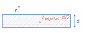
Select an option from the Offset definition list—
No offset (the default),
Physical offset, or
Relative offset. The default
No offset means that the modeled boundary coincides with the shell midsurface.
|
•
|
For Physical offset enter a value or expression in the zoffset field for the actual distance from the meshed boundary to the shell midsurface. 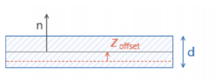
|
|
•
|
For Relative offset enter a value or expression in the zrel_offset field for the offset as the ratio between the offset distance and half the shell thickness. A value of +1 means that the actual shell bottom surface is located on the meshed boundary, and a value of −1 means that the shell top surface is located on the meshed boundary.
|
From the Structural transient behavior list, select
Include inertial terms (the default) or
Quasi-static. Use
Quasi-static to treat the dynamic behavior as quasi-static (with no mass effects; that is, no second-order time derivatives). Selecting this option gives a more efficient solution for problems where the variation in time is slow when compared to the natural frequencies of the system. The default solver for the time stepping is changed from Generalized alpha to BDF when
Quasi-static is selected.
Enter the default coordinates for the Reference point for moment computation xref. The resulting moments (applied or as reactions) are then computed relative to this reference point. During the results and analysis stage, the coordinates can be changed in the
Parameters section in the result nodes.
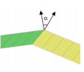
The fold-line limit angle α is the smallest angle between the normals of two boundaries that makes their intersection to be treated as a fold line. The normal to the shell is discontinuous along a fold-line. Enter a value or expression in the
α field. The default value is 0.05 radians (approximately 3 degrees). The value must be larger than 0, and less than
π/2, but angles larger than a few degrees are not usually meaningful.
Enter a number between -1 and 1 for the Local z-coordinate [-1,1] for thickness-dependent results Z. The value can be changed from
−1 (downside) to
+1 (upside). The default is +1. A value of 0 means the midsurface of the shell. This is the default position for stress and strain evaluation during the results analysis. During the results and analysis stage, the coordinates can be changed in the
Parameters section in the result features.
To display this section, click the Show button (

) and select
Advanced Physics Options. Normally these settings do not need to be changed.
The Use MITC interpolation check box is selected by default, and this interpolation, which is part of the MITC shell formulation, should normally always be active.
For the Plate interface, the Use 3D formulation check box is used to select whether six or three variables are used in the formulation. For geometrically nonlinear analyses, or when in-plane (membrane) forces are active, six variables must be used. This check box is selected by default.
If the Solve for out-of-plane strain components check box is selected, extra degrees of freedom will be added for computing the out-of-plane strain components. This formulation is similar to what is used for plane stress in the Solid Mechanics and Membrane interfaces and it is computationally somewhat more expensive than the standard formulation. In the default formulation, the out-of-plane strain in the shell is explicitly computed from the stress. This may cause circular references of variables if you for example want the constitutive law to be strain dependent. If you encounter such problems, use the alternative formulation.
To display this section, click the Show button (

) and select
Discretization.
Select the order of the Displacement field —
Linear or
Quadratic. The degrees of freedom for the displacement of the shell normals will always have the same shape functions as the displacements.
Both interfaces define two dependent variables (fields)—the displacement field u and the field of normal displacements
ar. The names can be changed but the names of fields and dependent variables must in general be unique within a model. If you intentionally use the same name for fields from different physics interfaces, these degrees of freedom are treated as being the same. This can be used when mixing different type of structural mechanics interfaces, where you often want the displacements to be the equal.