Computing Monochromatic Aberrations

The plot and the derived values node are used to analyze the performance of lens systems within the limit of the geometrical optics approach. In order to use the plot, the following prerequisites must be met:

•

The model component must be 3D.

•

An instance of the Geometrical Optics interface must be present and solved for.

•

The check box must be selected in the Geometrical Optics window before solving.

•

An data set must be created. This data set must point to a data set.

•

In the Settings window for the data set, must be selected from the list. The is the location of the focus and the points from the focus toward the center of the exit pupil.

Using the hemisphere defined in the data set, a Gaussian reference sphere is defined.

Zernike Polynomials

A standard way to quantify monochromatic aberrations is to express the optical path difference of all incident rays as a linear combination of Zernike polynomials.

Several different standards exist for naming, normalizing, and organizing the Zernike polynomials. The approach used in this section follows the standards published by the International Organization for Standardization (ISO, Ref. 2) and the American National Standards Institute (ANSI, Ref. 3).

Each Zernike polynomial

can be expressed as

where

•

is the normalization term,

•

is the radial term,

•

is the meridional term or azimuthal term,

•

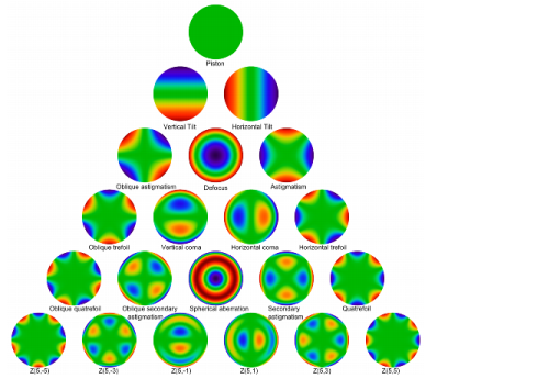
ρ is the radial parameter, given by ρ = r/a where r is the distance from the aperture center and a is the aperture radius, so that 0 ≤ ρ ≤ 1,

•

θ is the meridional parameter or azimuthal angle, 0 ≤ θ ≤ 2π,

•

the lower index n is a nonnegative integer, n = 0,1,2…, and

•

the upper index m is an integer, m = -n,-n+2…n-2,n so that

is always even.

The normalization term

where

is the Kronecker delta,

The radial term is given by the equation

where “!” denotes the factorial operator; for nonnegative integers,

The meridional term is given by the equation

The Zernike polynomials thus defined are normalized Zernike polynomials. They are orthogonal in the sense that any pair of Zernike polynomials satisfy the equation

The normalized Zernike polynomials up to fifth order, along with their common names, are given in Table 2-1.

Table 2-1: Zernike Polynomials
Term	Expression	Common Name
		Piston
		Vertical tilt
		Horizontal tilt
		Oblique astigmatism
		Defocus
		Astigmatism
		Oblique trefoil
		Vertical coma
		Horizontal coma
		Horizontal trefoil
		Oblique trefoil
		Oblique secondary astigmatism
		Spherical aberration
		Secondary astigmatism
		Horizontal trefoil

	‡
	†
	†
	‡