Quantities Computed by the Geometrical Optics Interface

By default, the Geometrical Optics interface declares dependent variables for the components of the ray position and wave vector. It is possible to define first-order differential equations for other dependent variables to be integrated over time or along the trajectory of each ray. An additional variable used to solve a user-defined first-order equation is called an Auxiliary Dependent Variable. It is possible to add an arbitrary number of auxiliary dependent variables to the Geometrical Optics interface, resulting in an arbitrary number of first-order equations being solved.

In addition, several quantities that are often of interest in geometrical optics applications, such as intensity and phase, are computed using built-in auxiliary dependent variables that can be activated by selecting certain options in the physics interface node’s Settings window.

The following sections describe the quantities that can be computed by changing settings in the Geometrical Optics interface.

Intensity Calculation

The calculation of ray intensity is controlled by the setting in the section of the physics interface node’s Settings window. The intensity is computed when the is set to , , , or .

When the ray intensity is computed, settings for specifying the initial ray intensity, wavefront shape, and polarization become available in all release features. It is possible to release polarized, unpolarized, and partially polarized rays. It is also possible to define the wavefront shape so that the ray intensity varies like that of a plane wave, spherical wave, or a wavefront with user-defined principal radii of curvature. These radii of curvature dictate whether the electromagnetic waves are converging or diverging, and the distance to the nearest focus (within the limits of the geometrical optics approximation).

The intensity of a ray is computed using four Stokes parameters that provide the flexibility to specify arbitrary states of polarization when releasing rays. The four Stokes parameters describe the ray intensity that would be observed by sending rays through certain combinations of polarizers and wave retarders. A comprehensive definition of the Stokes parameters is available in The Stokes Parameters in Theory for the Geometrical Optics Interface.

While the Stokes parameters determine the state of polarization of the rays, the magnitude of the intensity also depends on the degree to which a wavefront is converging or diverging. This information is stored by computing the principal radii of curvature of the wavefront. For more information on wavefront radii of curvature, see Principal Radii of Curvature in Theory for the Geometrical Optics Interface.

Altogether, to compute the intensity of a wavefront in 3D using the method of principal curvatures, a total of 11 additional degrees of freedom are defined per ray, including the following:

•

Four Stokes parameters,

•

Two principal radii of curvature,

•

Two initial principal radii of curvature, and

•

Three components of a unit vector that is used to define a local coordinate system with respect to which the Stokes parameters are defined.

Information about the local coordinate system is needed because such a coordinate system must often undergo transformations when rays interact with boundaries. The coefficients of reflection and transmission depend on the orientation of the electric field of the incident ray with respect to the plane of incidence. In addition, when rays interact with curved boundaries, the reinitialized radii of curvature of the reflected and refracted rays depend on the curvature and orientation of the boundaries.

In 2D, only the four Stokes parameters, one principal radius of curvature, and one initial principal radius of curvature are required, for a total of 6 additional degrees of freedom per ray. The out-of-plane radius is assumed to be arbitrarily large, so all of the rays correspond to planar or cylindrical wavefronts.

In 2D axisymmetric models, the four Stokes parameters, two principal radii of curvature, and two initial principal radii of curvature are allocated for each ray, for a total of 8 additional degrees of freedom per ray. The in-plane and out-of-plane radii of curvature are both permitted to change, allowing rays to interact with boundaries as if they were surfaces of revolution having both in-plane and out-of-plane curvature.

If is selected, the information about ray intensity and polarization is computed using a total of 8 degrees of freedom in 3D or 5 degrees of freedom in 2D. However, the method of principal curvatures is recommended in most cases, despite requiring more degrees of freedom, because the solution is more accurate when the time step taken by the solver is large. The main advantage of the option is that it can be used to compute the ray intensity in graded media, in which the refractive index changes continuously, whereas the option is only valid in homogeneous media, where the refractive index is constant within each domain and only changes during ray-boundary interactions.

Optical Path Length Calculation

It is possible to define an auxiliary dependent variable for the optical path length by selecting the check box in the section of the physics interface node’s Settings window. Initially the optical path length is set to 0 for all released rays. It is possible to reset the optical path length to 0 when the rays interact with boundaries.

Phase Calculation

The phase of a ray is necessary for some applications that require information about the instantaneous electric fields of multiple rays, such as interferometers. To define an auxiliary dependent variable for phase, select the check box in the section of the physics interface node’s Settings window. This check box is only available if the ray intensity is computed.

Because enabling the phase allows the instantaneous electric field of a ray to be plotted, phase calculation can be used to visualize the state of polarization of a system of rays.

Figure 2-2: Polarization of the reflected and refracted rays when an unpolarized ray crosses a material discontinuity at the Brewster angle, visualized using a Deformation node.

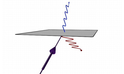
As shown in Figure 2-2, the polarization of a ray can be visualized when the free-space wavelength is sufficiently large by applying a node to a plot. A deformation proportional to the electric field can then be applied to the rays. The color expression corresponds to the degree of polarization of each ray; because the angle of incidence is equal to the Brewster angle, the reflected ray is completely polarized whereas the refracted ray is not.

Allow Frequency Distributions at Release Features

By default, the ray frequency or free-space wavelength is defined in the Ray Properties Settings window and has the same value for all rays. For some applications, however, it may be useful to model ray propagation over a wide range of frequency values. This can be accomplished by defining a parameter for the ray frequency and adding a to the study, but it is often more efficient to model the propagation of rays with a wide range of frequency values simultaneously. This can be accomplished by selecting the check box in the section of the physics interface node’s Settings window.

Selecting the check box causes an auxiliary dependent variable to be defined for the ray frequency, enabling a unique frequency value to be assigned to each ray. In the Settings windows for release features it is possible to release either a single ray of a specified frequency or a distribution of frequency values.


	Czerny-Turner Monochromator: Application Library path Ray_Optics_Module/Polychromatic_Light/czerny_turner_monochromator

Computing Deposited Ray Power

The total power transmitted by a ray depends on the ray intensity and the solid angle subtended by the wavefront. Although the former is computed when the is set to or in the section of the physics interface node’s Settings window, the latter is not.

It is possible to model heat generation on domains or boundaries due to the attenuation or absorption of rays by setting to or . In addition to the auxiliary dependent variables for the Stokes parameters, principal radii of curvature, and principal curvature direction, this option defines a variable for the total power transmitted by a ray. The changes in total ray power due to propagation in absorbing media and interaction with material discontinuities are proportional to the corresponding changes in the ray intensity. However, unlike the ray intensity, the total ray power is unaffected by changes in the principal radii of curvature.

When the variable for total ray power is computed, it is possible to compute the boundary heat source that is created when rays are absorbed at surfaces using the Deposited Ray Power (Boundary) subnode. In addition, if rays propagate through absorbing media, it is possible to model the changes in ray intensity and power and to compute the heat source resulting from the attenuation of rays. This heat source is automatically used to compute the temperature when The Ray Heating Interface is used. Alternatively, the coupling can be set up manually using the Ray Heat Source multiphysics node.

Corrections for Strongly Absorbing Media

The classical implementation of Snell’s law and the Fresnel equations is valid for ray propagation between media that are non-absorbing or weakly absorbing, meaning that the imaginary part of the refractive index is much smaller in magnitude than the real part of the refractive index. In such cases it can be assumed that the surface in which ray amplitude is constant and the surface in which ray phase is constant are both normal to the direction of ray propagation.

However, in strongly absorbing media, the surfaces of constant amplitude and surfaces of constant phase are not always parallel to each other. As a result, corrections to Snell’s law and the Fresnel equations are required. These corrections can be enabled by selecting the check box in the section of the physics interface node’s Settings window. This check box is only available if the ray intensity is computed. To store information about the orientation of the surfaces of constant phase, selecting this check box causes three auxiliary dependent variables to be declared in 3D models or two auxiliary dependent variables in 2D models.

Dependent Variables Created by Physics Features

The following dependent variables are created by adding specific physics features to the Geometrical Optics interface and changing their settings.

Initial Perturbation for Illuminated Surfaces

The Illuminated Surface feature includes an option to perturb the initial ray direction in order to model the effects of surface roughness. When the check box is selected in the settings window for at least one feature, an auxiliary dependent variable is declared. This auxiliary dependent variable is used to initialize the perturbed ray direction vectors.

Total Power Transmitted and Reflected at Gratings

The Grating feature is used to model the transmission and reflection of rays at diffraction gratings. It includes a Diffraction Order subnode that can be used to release secondary rays of nonzero diffraction order. When the is set to or in the section of the physics interface settings window, the and check boxes are shown in the settings window. Selecting either of these check boxes causes an auxiliary dependent variable to be declared, storing the total power of the transmitted and reflected rays of all diffraction orders.


	Diffraction Grating: Application Library path Ray_Optics_Module/Tutorials/diffraction_grating

Order of Initialization of Auxiliary Dependent Variables

When rays are released, the variables defined for each ray are initialized in a specific order. The initial values of ray variables can only depend on the values of variables that have already been defined. The order of dependent variable initialization is governed by the following rules:

•

The initial ray position is always determined first.

•

By default, user-defined auxiliary dependent variables (that is, those that are defined by adding an Auxiliary Dependent Variable node to the physics interface) are initialized after all other variables. They can instead be initialized immediately after the ray position vector components by selecting the check box shown in all release features.

Figure 2-3: Settings for initializing auxiliary dependent variables before or after other degrees of freedom.

•

If more than one user-defined auxiliary dependent variable is present, these variables are initialized in the order in which the corresponding nodes appear in the Model Builder.

•

The remaining degrees of freedom are defined in the following order (each listed group is initialized simultaneously, and the variables within a group cannot reliably be initialized in terms of each other):

Help variable for the perturbation of initial ray direction at illuminated surfaces,

Ray frequency,

The wave vector components, optical path length, and total power transmitted and reflected by gratings,

The components of the unit vector that indicates the direction corresponding to one of the principal radii of curvature,

The principal radii of curvature, initial principal radii of curvature, the initial Stokes parameters, and help variables for computing the curvature tensor and intensity, and

The total power transmitted by the ray.

For example, the initial ray direction vector may depend on the ray frequency, but the initial principal radii of curvature may not depend on the total power transmitted by the ray.