Common Study Step Settings

The study steps form a solver configuration that computes the solutions for the study. The study step nodes’ windows contain the following sections (in addition to specific study settings for each type of study step):

On top of the study steps windows, a toolbar contains the following commands:

If you have a license for the Acoustics Module, MEMS Module, or Structural Mechanics Module (including any add-on modules such as the Nonlinear Structural Materials Module) and your model involves structural mechanics, then the section includes an check box.

Select the check box to enable a geometrically nonlinear analysis for the study step. Some physics designs force a geometrically nonlinear analysis, in which case it is not possible to clear the check box. For further details, see the theory sections for the respective physics interface in the applicable modules’ manuals.

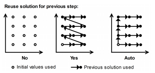
Select an option from the list.

•

(the default for a Stationary study) to reset the solution to the initial values before each step or continuation sweep. The initial values will not be recalculated by the parametric solver for subsequent parameter values. Parameter dependence of the initial values can be accomplished by using parametric sweep.

•

(the default for a Frequency Domain study) to normally use the converged solution from the previous step or sweep. However, when multiple parameters are used, the solution from the first step of each parameter list is always used for the first step of the next list.

The difference between the three options is shown in Figure 19-2 for a 3 x 4 two-parameter sweep using the different choices for without continuation:

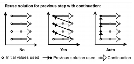
When continuation is enabled by setting to one of the parameters, the converged solutions are always reused for the steps along the continuation sweep in this parameter. The setting for then determines how the solutions are reused between multiple continuation sweeps, if there are additional parameters to sweep over, as shown in Figure 19-3.

For the Frequency Domain study, the auxiliary sweep is merged with the frequency sweep into a multiparameter sweep with the frequency as the parameter at the innermost level.

See About the Parametric Solver.

Select the check box to allow plotting of results while solving in the window. Then select what to plot from the list and, for time-dependent simulations, at which time steps to update the plot: the output times or the time steps taken by the solver. The software plots the data set of the selected plot group as soon as the results become available. You can also control which probes to tabulate and plot the values from. The default is to tabulate and plot the values from all probes in the window and a window.

Use the list to select any probes to evaluate. The default is , which selects all probes for plotting and tabulation of probe data. Select to open a list with all available probes. Use the (

), (

), and (

) buttons to make the list contain the probes that you want to see results from while solving. Select to not include any probe.

	You can use probes to tabulate values of interest during a large parametric simulation, for example. It can then be possible to keep only the last solution in memory during the parametric sweep, which potentially can significantly reduce memory requirements and the simulation time.

See Physics and Variables Selection for detailed information about this section. You can control and specify different cases where the physics interface to solve for is varied, or, for various analysis cases, which variables and physics features (for example, boundary conditions and sources) to use. The default is to solve for all physics interfaces that are compatible with the study type.

When you have physics interfaces in a study step that you do not solve for but that provide degrees of freedom, you can specify how the COMSOL software handles the values of such degrees of freedom (dependent variables).

The settings in this section determine how the solver handles dependent variables that you do not solve for. This is applicable in, for example, a solver configuration where you only solve for a subset of the dependent variables in each step. You can also specify the initial values of variables that you do solve for.

By default, COMSOL Multiphysics determines these values heuristically depending on the physics as, for example, the specified initial values or a solution from an earlier study step. Under , the default value of the list is . To specify the initial values of the dependent variables that you solve for, select from the list.

	The Initial values of variables solved for settings have no effect when using the eigenvalue solver.

Then use the list to specify how to compute the initial values of variables solved for and the values of variables not solved for. Select:

Use the list to specify what study to use if has been set to :

Depending on the study type of the solution that you selected, you can choose different solutions from a list underneath the list:

•

For a Stationary study, from the list, select (the default) to use the last (typically the only) solution, select to use the first (typically the only) solution, select to use the last (typically the only) solution, select to use all (typically just one) solutions from that study, select to use a specific solution number that you specify, or select to use the first (typically the only) solution. If you use a parametric continuation of the stationary study, there can be additional solutions to choose from.

•

For a Time Dependent study, from the list, select (the default) to use the solution for the last time, select to use the first solution, select to use the last solution, select to use all solutions from that study, select to specify a time in the text field that opens and use the interpolated solution at that time, select to use a specific solution number that you specify, or select one of the output times to use the solution at that time. For all the options in the list (except ), one solution is used throughout the whole simulation. This solution is computed once before the simulation. When you select , an interpolation is done internally for time-dependent simulations.

•

For an Eigenvalue study, from the list, select (the default) to use the first eigenvalue and its associated eigensolution, select to use the first solution, select to use the last solution, select to use all solutions from that study, select to use a specific solution number that you specify, or select one of the eigenvalues to use the corresponding eigensolution.

•

For a parametric or Frequency Domain study, from the list, select (the default) to use the first parameter value set or frequency, select to use the first solution, select to use the last solution, select to use all solutions from that study, select to use a specific solution number that you specify, or select one of the parameter value sets or frequencies to use the corresponding solution.

	The All option is not available from the list under Initial values of variables solved for.

Under , you can specify to store the field variables that you solve only for some part of the geometry (a boundary, for example, if the solution in the domain is not of interest). You define the parts of the geometry for which to store the fields as selection nodes. From the list, choose (the default) to store all fields in all parts of the geometry where they are defined, or choose For selections to choose one or more selections that you add to the list. Click the button (

) to open an dialog box that contains all available selections. Select the selections that you want to add and then click . You can also delete selections from the list using the button (

) and move them using the (

) and (

) buttons. See also the Field node, where you can also control what to store in the output, if the corresponding Dependent Variables uses user-defined settings.

Specify — for each geometry — which mesh to use for the study step. For each geometry listed in the column, select a mesh from the list of meshes in the column. Each list of meshes contains the meshes defined for the geometry that you find on the same row.

These are settings for mesh adaptation and error estimates, available for stationary, eigenfrequency, eigenvalue, and frequency-domain study steps. Depending on the type of adaptation, meshing sequences for the adaptive mesh refinements, using or nodes, and corresponding solutions are created for inspection and possible modification. Error estimates are available as variables for postprocessing (for example, freq.errtot for the total error estimate in a Frequency Domain study).

From the list, select if you want to use error estimation and select if you want to use adaptive mesh refinement. In the latter case, error estimates that are used in the adaptation algorithm are also available for postprocessing. Choose for no adaptation or error estimation.

The software performs adaptive mesh refinement in one geometry only. Use the list to specify that geometry.

Use the list to control how the error estimate is computed. Select to use the squared L2 norm of the error. This is the only option for Eigenvalue studies. Select and specify a . Available functional types are and . This option adapts the mesh toward improved accuracy in the expression for the functional. Select to specify a globally available scalar-valued expression. If you select , you can choose a ( when doing error estimation) from the following list:

The field is only available for set to . Use this field to enter a space-separated list of scaling factors, one for each field variable (default: 1). The error estimate for each field variable is divided by this factor.

From the list, select which solution that should be used to evaluate error estimates:

In the field (only available when is or ), enter weights as a space-separated list of positive (relative) weights so that the error estimate is a weighted sum of the error estimates for the various solutions (eigenmodes). The default value of 1, which means that all the weight is put on the first solution (eigenmode). That is, any omitted weight components are treated as zero weight.

From the list (only available when is ), select an error estimate method in the adjoint solution: a recovery technique or a gradient-based method. Select (the default) to enforce using the recovery technique when possible, and select to use the gradient-based method.

The check box is selected per default. Clear this check box if you do not want to save solution on every refined mesh. In that case the last two solutions are saved (the finest one and the second finest).

Under , the following settings are available.

Use the list to control how to refine mesh elements. Select on of these options:

The field is only available when is ). The size of the refined mesh is the minimum of the size of the original mesh (previous refined mesh) and the size defined by the refinement. Specify the (a value of 3 by default) to scale the refined mesh size in the regions where refinement is not needed.

By default, the software automatically determines the order of decrease in equation residuals on basis of the shape function orders in the geometry. To specify a residual order manually, select the check box and specify a nonnegative integer in the accompanying field. Use the list to specify how the solver should select which elements to refine. Select:

•

to minimize the error by refining a fraction of the elements with the largest error in such a way that the total number of elements increases roughly by the factor specified in the accompanying field. The default value is 1.7, which means that number of elements increases by about 70%.

•

to refine elements whose local error indicator is larger than a given fraction of the largest local error indicator. Use the accompanying field to specify the fraction. The default value is 0.5, which means that the fraction contains the elements with more than 50% of the largest local error.

•

to refine a given fraction of the elements. Use the accompanying field to specify the fraction. The default value is 0.5, which means that the solver refines about 50% of the elements.

Use the field to specify the maximum number of refinement iterations. The default value is 2.

Use the field to specify the maximum number of elements in the refined mesh. If he number of elements exceeds this number, the solver stops even if it has not reached the number specified in the field.

These are extensions to the study’s main solver, such as adaptive mesh refinement and automatic remeshing. The options vary depending on the study type.

Select the check box to enable an auxiliary parameter sweep, which corresponds to a Parametric solver attribute node. For each set of parameter values, the chosen is solved for. This is available for Stationary, Time Dependent, and Frequency Domain studies.

Select a to specify the type of sweep to perform:

•

(the default) solves for a number of given combinations of values as given for each parameter in the list. The parameter lists are combined in the order given, that is, the first combination contains the first value in each list, the second combination contains all second values, and so on.

•

solves for all combinations of values; that is, all values for each parameter are combined with all values for the other parameters. Using all combinations can lead to a very large number of solutions (equal to the product of the lengths of the parameter lists).

In the table, specify the , , and (optional) for the parametric solver. Click the button (

) to add a row to the table. When you click in the column to define the parameter values, click the button (

) to define a range of parameter values. The parameter unit overrides the unit of the global parameter. If no parameter unit is given, parameter values without explicit dimensions are considered dimensionless.

	If you choose Specified combinations, the list of values must have equal length.

An alternative to specifying parameter names and values directly in the table is to specify them in a text file. Use the button (

) to browse to such a text file. The read names and values are appended to the current table. The format of the text file must be such that the parameter names appear in the first column and the values for each parameter appear row-wise with a space separating the name and values and a space separating the values.