Far Field

•

For the RF Module and the Wave Optics Module, the variables are the far-field norm, normEfar and normdBEfar; the components of the far-field variable Efar; and the axial ratio, axialRatio and axialRatiodB.

The variables are plotted for a selected number of angles on a circle (in 2D) or a sphere (in 3D). The angle interval and the number of angles can be manually specified. Also the circle origin and radius of the circle (2D) or sphere (3D) can be specified. For 3D Far Field plots, you also specify an expression for the surface color. For 1D Far Field plots, you can optionally compute the beam width.

The far-field plot plots a surface shape by deforming the specified circle or sphere in 2D and 3D, or a circular slice in 1D. For each evaluation point on the specified circle or sphere, the plot deforms the specified circle or sphere from the evaluation point in the radial direction so that the deformed surface shape distance from the origin becomes equal to the value of the specified expression on the evaluation point on the specified circle or sphere.

The main advantage with the Far Field plot, as compared to making a Line Graph, is that the circle or sphere used for defining the plot directions is not part of the geometry for the solution. Thus, the number of plotting directions is decoupled from the discretization of the solution domain.

To add this plot type, right-click a plot group node and choose from the menu.

	Go to Common Results Node Settings for links to information about these sections: Data, Title, Range, Inherit Style, and Coloring and Style. For 3D plot groups, see the list for Color. For Far Field plots, only Solution data sets are available as inputs.

For the standard settings, see Expressions and Predefined Quantities. In 3D, you can also select the check box and then enter a threshold value as a scalar number in the associated edit field. The threshold value corresponds to the evaluated radius that maps to the plotted radius 0. The default, if the check box is cleared, is the minimum radius among those evaluated for. Additionally, in 3D, select the check box to use the far-field plot expression defined in this section also as the color expression. The section is then not available.

Under , enter the . The default is 50.

Select a : (the default) or . If is selected, enter values (SI unit: deg) for

(the default is 0 degrees) and

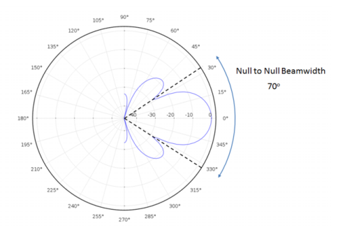
(the default is 360 degrees). If you want to compute the beam width, select from the list. Then, a field appears, where you can specify a nonnegative number to compute the beam width at a certain level down from the reference direction. The unit for that level is the same as the unit for the expression used in the far-field plot (dB, for example, for a far-field sound pressure level). The beam width is the width of the lobe around the reference direction (in degrees). When you compute the beam width, the computed values appear in a table with columns for the parameter (typically a frequency), the beam width, and the null-to-null beam width (the angular separation from which the magnitude of the radiation pattern decreases to zero away from the main beam; see the figure below).

Note that the beam width calculation only makes sense if there is a main lobe in the reference direction.

For 1D Far Field plot nodes referring to a solution in a 2D axisymmetric or 3D component, under enter the coordinate at the center of the evaluation circle. Under specify the normal to the circular slice of the far-field bulb. The defaults is {0, 0, 1} for the normal using 3D components and {0, 1, 0} for the normal using 2D axisymmetric components.

If a pressure acoustics interface is used in the component from which the data set is taken, you can also add a (SI unit: m) under for a radius-dependent far-field expression.

Under specify a reference direction from which the angle is measured. The entered vector is projected onto the evaluation plane. The default is {1, 0, 0} for the reference direction using 3D components and {0, 0, 1} for the reference direction using 2D axisymmetric components.

A schematic of the evaluation circle is depicted in Figure 20-3. In 3D, you can preview the evaluation circle in the geometry by clicking the at the bottom of the section. An example of the resulting plot is depicted in Figure 20-4.

Under , enter the . The default is 10. Enter the . The default is 20.

Select a : (the default) or . If is selected in a 3D plot group, you can also select the check box. If the check box is selected, you can enter or select an expression for the directivity in the field. The direction for the strongest radiation and the directivity value (also in dB) display in a table window (see The Table Window and Tables Node). So if, for example, you model a speaker that is located in an infinite baffle (and symmetry is used in the far-field calculation), then plot and evaluate the whole field to get the directivity.

If is selected, enter values (SI unit: deg) for:

If a pressure acoustics interface is used in the component from which the data set is taken, you can also specify the following settings for a radius-dependent far-field expression. Under from the list, select (the default) or . If is selected, enter values for the , , and coordinates at the center of the sphere (SI unit: m). The default is 0. Enter a (SI unit: m). The default is 1 m.

This section is available in 1D plot groups only. Select the check box to display the plotted expressions to the right of the plot. In plots where each line represents a certain time value, eigenvalue, or parameter value, these values are also displayed.

When is selected from the list (the default), the legend texts appear automatically. You can add a prefix or a suffix to the automatic legend text in the and fields. If is selected from the list, enter your own legend text into the table.